The PHREG Procedure

Classical Method of Maximum Likelihood

PROC PHREG fits the Cox model by maximizing the partial likelihood and computes the baseline survivor function by using the Breslow (1972) estimate. The following statements produce Figure 85.1 and Figure 85.2:

ods graphics on;
proc phreg data=Rats plot(overlay)=survival;
   model Days*Status(0)=Group;
   baseline covariates=regimes out=_null_;
run;

In the MODEL statement, the response variable, Days, is crossed with the censoring variable, Status, with the value that indicates censoring is enclosed in parentheses. The values of Days are considered censored if the value of Status is 0; otherwise, they are considered event times.

Graphs are produced when ODS Graphics is enabled. The survival curves for the two observations in the data set Regime, specified in the COVARIATES= option in the BASELINE statement, are requested through the PLOTS= option with the OVERLAY option for overlaying both survival curves in the same plot.

Figure 85.2 shows a typical printed output of a classical analysis. Since Group takes only two values, the null hypothesis for no difference between the two groups is identical to the null hypothesis that the regression coefficient for Group is 0. All three tests in the "Testing Global Null Hypothesis: BETA=0" table (see the section Testing the Global Null Hypothesis) suggest that the survival curves for the two pretreatment groups might not be the same. In this model, the hazard ratio (or risk ratio) for Group, defined as the exponentiation of the regression coefficient for Group, is the ratio of the hazard functions between the two groups. 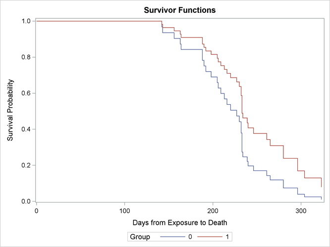The estimate is 0.551, implying that the hazard function for Group=1 is smaller than that for Group=0. In other words, rats in Group=1 lived longer than those in Group=0. This conclusion is also revealed in the plot of the survivor functions in Figure 85.2.

Figure 85.1: Comparison of Two Survival Curves

The PHREG Procedure

Model Information
Data Set	WORK.RATS
Dependent Variable	Days	Days from Exposure to Death
Censoring Variable	Status
Censoring Value(s)	0
Ties Handling	BRESLOW

Number of Observations Read

Number of Observations Used

Summary of the Number of Event and Censored Values
Total	Event	Censored	Percent Censored
40	36	4	10.00

Convergence Status
Convergence criterion (GCONV=1E-8) satisfied.

Model Fit Statistics
Criterion	Without Covariates	With Covariates
-2 LOG L	204.317	201.438
AIC	204.317	203.438
SBC	204.317	205.022

Testing Global Null Hypothesis: BETA=0
Test	Chi-Square	DF	Pr > ChiSq
Likelihood Ratio	2.8784	1	0.0898
Score	3.0001	1	0.0833
Wald	2.9254	1	0.0872

Analysis of Maximum Likelihood Estimates
Parameter	DF	Parameter Estimate	Standard Error	Chi-Square	Pr > ChiSq	Hazard Ratio
Group	1	-0.59590	0.34840	2.9254	0.0872	0.551

Figure 85.2: Survivorship for the Two Pretreatment Regimes

In this example, the comparison of two survival curves is put in the form of a proportional hazards model. This approach is essentially the same as the log-rank (Mantel-Haenszel) test. In fact, if there are no ties in the survival times, the likelihood score test in the Cox regression analysis is identical to the log-rank test. The advantage of the Cox regression approach is the ability to adjust for the other variables by including them in the model. For example, the present model could be expanded by including a variable that contains the initial body weights of the rats.

Next, consider a simple test of the validity of the proportional hazards assumption. The proportional hazards model for comparing the two pretreatment groups is given by the following:

$\lambda (t)=\left\{ \begin{array}{ll} \lambda _{0}(t) & \mbox{ if GROUP}=0 \\ \lambda _{0}(t)e^{\beta _{1}} & \mbox{ if GROUP}=1 \end{array} \right.$

The ratio of hazards is $e^{\beta _{1}}$ , which does not depend on time. If the hazard ratio changes with time, the proportional hazards model assumption is invalid. Simple forms of departure from the proportional hazards model can be investigated with the following time-dependent explanatory variable $x=x(t)$ :

$x(t) = \left\{ \begin{array}{ll} 0 & \mbox{ if GROUP}=0 \\ \log (t)-5.4 & \mbox{ if GROUP}=1 \end{array} \right.$

Here, $\mr{log}(t)$ is used instead of t to avoid numerical instability in the computation. The constant, 5.4, is the average of the logs of the survival times and is included to improve interpretability. The hazard ratio in the two groups then becomes $e^{ \beta _{1}-5.4\beta _{2}} t^{\beta _{2}}$ , where $\beta _{2}$ is the regression parameter for the time-dependent variable x. The term $e^{ \beta _{1}}$ represents the hazard ratio at the geometric mean of the survival times. A nonzero value of $\beta _{2}$ would imply an increasing $(\beta _{2}>0)$ or decreasing $(\beta _{2}<0)$ trend in the hazard ratio with time.

The following statements implement this simple test of the proportional hazards assumption. The MODEL statement includes the time-dependent explanatory variable X, which is defined subsequently by the programming statement. At each event time, subjects in the risk set (those alive just before the event time) have their X values changed accordingly.

proc phreg data=Rats;
   model Days*Status(0)=Group X;
   X=Group*(log(Days) - 5.4);
run;

The analysis of the parameter estimates is displayed in Figure 85.3. The Wald chi-square statistic for testing the null hypothesis that $\beta _{2}=0$ is 0.0158. The statistic is not statistically significant when compared to a chi-square distribution with one degree of freedom (p = 0.8999). Thus, you can conclude that there is no evidence of an increasing or decreasing trend over time in the hazard ratio.

Figure 85.3: A Simple Test of Trend in the Hazard Ratio

The PHREG Procedure

Analysis of Maximum Likelihood Estimates
Parameter	DF	Parameter Estimate	Standard Error	Chi-Square	Pr > ChiSq	Hazard Ratio
Group	1	-0.59976	0.34837	2.9639	0.0851	0.549
X	1	-0.22952	1.82489	0.0158	0.8999	0.795