The PHREG Procedure
- Overview
-
Getting Started

-
SyntaxPROC PHREG StatementASSESS StatementBASELINE StatementBAYES StatementBY StatementCLASS StatementCONTRAST StatementEFFECT StatementESTIMATE StatementFREQ StatementHAZARDRATIO StatementID StatementLSMEANS StatementLSMESTIMATE StatementMODEL StatementOUTPUT StatementProgramming StatementsRANDOM StatementSTRATA StatementSLICE StatementSTORE StatementTEST StatementWEIGHT Statement
-
DetailsFailure Time DistributionTime and CLASS Variables UsagePartial Likelihood Function for the Cox ModelCounting Process Style of InputLeft-Truncation of Failure TimesThe Multiplicative Hazards ModelProportional Rates/Means Models for Recurrent EventsThe Frailty ModelProportional Subdistribution Hazards Model for Competing-Risks DataHazard RatiosNewton-Raphson MethodFirth’s Modification for Maximum Likelihood EstimationRobust Sandwich Variance EstimateTesting the Global Null HypothesisType 3 Tests and Joint TestsConfidence Limits for a Hazard RatioUsing the TEST Statement to Test Linear HypothesesAnalysis of Multivariate Failure Time DataModel Fit StatisticsSchemper-Henderson Predictive MeasureResidualsDiagnostics Based on Weighted ResidualsInfluence of Observations on Overall Fit of the ModelSurvivor Function EstimatorsCaution about Using Survival Data with Left TruncationEffect Selection MethodsAssessment of the Proportional Hazards ModelThe Penalized Partial Likelihood Approach for Fitting Frailty ModelsSpecifics for Bayesian AnalysisComputational ResourcesInput and Output Data SetsDisplayed OutputODS Table NamesODS Graphics
-
ExamplesStepwise RegressionBest Subset SelectionModeling with Categorical PredictorsFirth’s Correction for Monotone LikelihoodConditional Logistic Regression for m:n MatchingModel Using Time-Dependent Explanatory VariablesTime-Dependent Repeated Measurements of a CovariateSurvival CurvesAnalysis of ResidualsAnalysis of Recurrent Events DataAnalysis of Clustered DataModel Assessment Using Cumulative Sums of Martingale ResidualsBayesian Analysis of the Cox ModelBayesian Analysis of Piecewise Exponential ModelAnalysis of Competing-Risks Data
- References
Proportional Subdistribution Hazards Model for Competing-Risks Data
Competing risks arise in the analysis of time-to-event data when the event of interest can be impeded by a prior event of a different type. For example, a leukemia patient’s relapse might be unobservable because the patient dies before relapse is diagnosed. In the presence of competing risks, the Kaplan-Meier method of estimating the survivor function is biased, because you can no longer assume that a subject will experience the event of interest if the follow-up period is long enough. The cumulative incidence function (CIF), which is the marginal failure subdistribution of a given cause, is widely used in competing-risks analysis.
The proportional hazards model for the subdistribution that Fine and Gray (1999) propose aims at modeling the cumulative incidence of an event of interest. They define a subdistribution hazard,
![\[ \bar{\lambda }_ k(t) = - \frac{d}{dt} \left(1 - F_ k(t) \right) \]](images/statug_phreg0286.png)
where  is the cumulative incidence function for the failure of cause k, and they impose a proportional hazards assumption on the subdistribution hazards:
![\[ \bar{\lambda }_ k(t|\bZ ) = \bar{\lambda }_{k,0} \exp (\bbeta _ k’\bZ ) \]](images/statug_phreg0288.png)
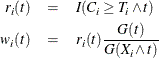
The estimation of the regression coefficients is based on modified risk sets, where subjects that experience a competing event are retained after their event. The weight of those subjects that are artificially retained in the risk sets is gradually reduced according to the conditional probability of being under follow-up had the competing event not occurred.
You use PROC PHREG to fit the Fine and Gray (1999) model by specifying the EVENTCODE= option in the MODEL statement to indicate the event of interest. Maximum likelihood estimates of the regression coefficients are obtained by the Newton-Raphson algorithm. The covariance matrix of the parameter estimator is computed as a sandwich estimate. You can request the CIF curves for a given set of covariates by using the BASELINE statement. The PLOTS=CIF option in the PROC PHREG statement displays a plot of the curves. You can obtain Schoenfeld residuals and score residuals by using the OUTPUT statement.
To model the subdistribution hazards for clustered data (Zhou et al. 2012), you use the COVS(AGGREGATE) option in the PROC PHREG statement. You also have to specify the ID statement to identify the clusters. To model the subdistribution hazards for stratified data (Zhou et al. 2011), you use the STRATA statement. PROC PHREG handles only regular stratified data that have a small number of large subject groups.
When you specify the EVENTCODE= option in the MODEL statement, the ASSESS, BAYES, and RANDOM statements are ignored. The ATRISK and COVM options in the PROC PHREG statement are also ignored, as are the following options in the MODEL statement: BEST=, DETAILS, HIERARCHY=, INCLUDE=, NOFIT, PLCONV=, RISKLIMITS=PL, SELECTION=, SEQUENTIAL, SLENTRY=, SLSTAY=, TYPE1, and TYPE3(LR, SCORE). Profile likelihood confidence intervals for the hazard ratios are not available for the Fine and Gray competing-risks analysis.
Parameter Estimation
For the ith subject,  , let
, let  ,
,  ,
,  , and
, and  be the observed time, event indicator, cause of failure, and covariate vector at time t, respectively. Assume that K causes of failure are observable (
 ). Consider failure from cause 1 to be the failure of interest, with failures of other causes as competing events. Let
Note that if  , then
 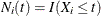 and
and  ; if
; if  , then
  and
and  . Let
. Let
where  is the Kaplan-Meier estimate of the survivor function of the censoring variable, which is calculated using
 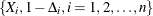 . If
. If  , then
  when
when  and 0 otherwise; and if
  , then . Table 85.12 displays the weight of a subject at a function of time.
Table 85.12: Weight for the ith Subject
|
|
Status |
|
|
|
|---|---|---|---|---|
|
|
|
1 |
1 |
1 |
|
|
1 |
1 |
1 |
|
|
|
1 |
1 |
1 |
|
|
|
|
0 |
1 |
0 |
|
|
1 |
0 |
|
|
|
|
1 |
1 |
|


The regression coefficients  are estimated by maximizing the pseudo-likelihood
  with respect to :
![\[ L(\bbeta ) = \prod _{i=1}^ n \left( \frac{\exp (\bbeta '\bZ _ i(X_ i))}{ \sum _{j=1}^ n Y_ j(X_ i)w_ j(X_ i) \exp (\bbeta '\bZ _ j(X_ i))}\right)^{I(\Delta _ i\epsilon _ i=1)} \]](images/statug_phreg0318.png)
The variance-covariance matrix of the maximum likelihood estimator  is approximated by a sandwich estimate.
With  ,
,  , and
, and  , let
, let
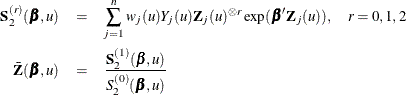
The score function  and the observed information matrix
  are given by
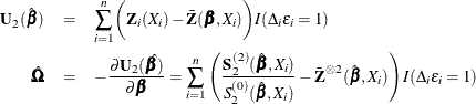
The sandwich variance estimate of is
![\[ \widehat{\mr{var}}(\hat{\bbeta }) = \hat{\bOmega }^{-1} \hat{\bSigma } \hat{\bOmega }^{-1} \]](images/statug_phreg0326.png)
where  is the estimate of the variance-covariance matrix of
  that is given by
![\[ \hat{\bSigma } = \sum _{i=1}^ n (\hat{\bm {\eta }}_ i + \hat{\bpsi }_ i)^{\otimes 2} \\ \]](images/statug_phreg0329.png)
where
![\[ \hat{\bm {\eta }}_ i = \int _0^\infty \biggl (\bZ _ i(u) - \bar{\bZ }(\hat{\bbeta },u) \biggr ) w_ i(u) d\hat{M}_ i^1(u) \]](images/statug_phreg0330.png)
![\[ \hat{\bpsi }_ i =\int _0^\infty \frac{\hat{\mb{q}}(u)}{\pi (u)} d\hat{M}_ i^ c(u) \]](images/statug_phreg0331.png)
![\[ \hat{\mb{q}}(u) = - \sum _{i=1}^{n} \int _0^\infty \biggl (\bZ _ i(s) - \bar{\bZ }(\hat{\bbeta }, s) \biggr ) w_ i(s)d\hat{M}_ i^1I(s\geq u > X_ i) \]](images/statug_phreg0332.png)
![\[ \pi (u) = \sum _ j I(X_ j \geq u) \]](images/statug_phreg0333.png)
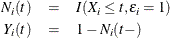
![\[ \hat{M}_ i^1(t) = N_ i(t) - \int _0^ t Y_ i(s) \exp (\hat{\bbeta }’\bZ _ i(s)) d\hat{\Lambda }_{10}(s) \]](images/statug_phreg0334.png)
![\[ \hat{M}_ i^ c(t) = I(X_ i \leq t, \Delta _ i=0) - \int _0^ t I(X_ i\geq u) d\hat{\Lambda }^ c(u) \]](images/statug_phreg0335.png)
![\[ \hat{\Lambda }_{10}(t) = \sum _{i=1}^ n \int _0^ t \frac{1}{S_2^{(0)}(\hat{\bbeta },u)} w_ i(u) dN_ i(u) \]](images/statug_phreg0336.png)
![\[ \hat{\Lambda }^ c(t) = \int _0^ t \frac{\sum _ i d\{ I(X_ i \leq u, \Delta _ i=0) \} }{\sum _ i I(X_ i \geq u)} \]](images/statug_phreg0337.png)
Residuals
You can use the OUTPUT statement to output Schoenfeld residuals and score residuals to a SAS data set.
|
Schoenfeld residuals: |
|
|
|
Score residuals |
|
|


Cumulative Incidence Prediction
For an individual with covariates  , the cumulative subdistribution hazard is estimated by
![\[ \hat{\Lambda }_1(t;\mb{z}_0) = \int _0^ t \exp [\hat{\bbeta }’\mb{z}_0]d\hat{\Lambda }_{10}(u) \]](images/statug_phreg0342.png)
and the predicted cumulative incidence is
![\[ \hat{F}_1(t;\mb{z}_0) = 1 - \exp [-\hat{\Lambda }_1(t;\mb{z}_0)] \]](images/statug_phreg0343.png)
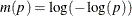
To compute the confidence interval for the cumulative incidence, consider a monotone transformation  with first derivative
  . Fine and Gray (1999, Section 5) give the following procedure to calculate pointwise confidence intervals. First, you generate B samples of normal random deviates
  . You can specify the value of B by using the NORMALSAMPLE= option in the BASELINE statement. Then, you compute the estimate of var
![$\{ m[\hat{F}_1(t;\bm {z}_0)] - m[F_1(t;\bm {z}_0)]\} $](images/statug_phreg0347.png) as
as
![\[ \hat{\sigma }^2(t;\bm {z}_0) = \frac{1}{B} \sum _{k=1}^ B \hat{J}_{1k}^2(t;\bm {z}_0) \]](images/statug_phreg0348.png)
where
![\begin{eqnarray*} \hat{J}_{1k}(t;\bm {z}_0) & = & \dot{m}[\hat{F}_1(t;\mb{z}_0)]\exp [- \hat{\Lambda }_1(t;\mb{z}_0)] \sum _{i=1}^ n A_{ki} \biggl \{ \int _0^ t \frac{\exp (\hat{\bbeta }'\bm {z}_0)}{S_2^{(0)}(\hat{\bbeta },u)} w_ i(u) d\hat{M}^1_ i(u) \\ & & + ~ \hat{\bm {h}}’(t;\bm {z}_0) \hat{\bOmega }^{-1}(\hat{\bm {\eta }}_ i + \hat{\bpsi }_ i) + \int _0^\infty \frac{\hat{\bm {v}}(u,t,\bm {z}_0)}{\hat{\pi }(u)} d\hat{M}_ i^ c(u) \biggr \} \end{eqnarray*}](images/statug_phreg0349.png)
![\[ \hat{\mb{h}}(t;\mb{z}_0) = \exp (\hat{\bbeta }’\mr{z}_0) \biggl \{ \hat{\Lambda }_{10}(t)\mb{z}_0 - \int _0^ t \bar{\bZ }(\hat{\bbeta },u)d\hat{\Lambda }_{10}(u) \biggr \} \]](images/statug_phreg0350.png)
![\[ \hat{v}(u,t,\mb{z}_0) = -\exp (\hat{\bbeta }’\mr{z}_0) \sum _{i=1}^ n \int _0^ t \frac{1}{S_2^{(0)}(\hat{\bbeta },s)} w_ i(s) d\hat{M}_ i^1(s) I(s \geq u > X_ i) \]](images/statug_phreg0351.png)
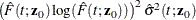
A 100(1– )% confidence interval for
  is given by
![\[ m^{-1} \biggl ( m[\hat{F}_1(t;\mb{z}_0)] \pm z_{\alpha } \hat{\sigma }(t;\mb{z}_0) \biggr ) \]](images/statug_phreg0353.png)
where  is the
  th percentile of a standard normal distribution.
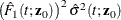
The CLTYPE option in the BASELINE statement enables you to choose the LOG transformation, the LOGLOG (log of negative log) transformation, or the IDENTITY transformation. You can also output the standard error of the cumulative incidence, which is approximated by the delta method as follows:
![\[ \hat{\sigma }^2(\hat{F}(t;\mb{z}_0)) = \left(\dot{m}[\hat{F}(t;\mb{z}_0)] \right)^{-2} \hat{\sigma }^2(t;\mb{z}_0) \]](images/statug_phreg0356.png)
Table 85.13 displays the variance estimator for each transformation that is available in PROC PHREG.
Table 85.13: Variance Estimate of the CIF Predictor
|
CLTYPE= keyword |
Transformation |
|
|---|---|---|
|
IDENTITY |
|
|
|
LOG |
|
|
|
LOGLOG |
|
|