The PHREG Procedure
- Overview
-
Getting Started

-
SyntaxPROC PHREG StatementASSESS StatementBASELINE StatementBAYES StatementBY StatementCLASS StatementCONTRAST StatementEFFECT StatementESTIMATE StatementFREQ StatementHAZARDRATIO StatementID StatementLSMEANS StatementLSMESTIMATE StatementMODEL StatementOUTPUT StatementProgramming StatementsRANDOM StatementSTRATA StatementSLICE StatementSTORE StatementTEST StatementWEIGHT Statement
-
DetailsFailure Time DistributionTime and CLASS Variables UsagePartial Likelihood Function for the Cox ModelCounting Process Style of InputLeft-Truncation of Failure TimesThe Multiplicative Hazards ModelProportional Rates/Means Models for Recurrent EventsThe Frailty ModelProportional Subdistribution Hazards Model for Competing-Risks DataHazard RatiosNewton-Raphson MethodFirth’s Modification for Maximum Likelihood EstimationRobust Sandwich Variance EstimateTesting the Global Null HypothesisType 3 Tests and Joint TestsConfidence Limits for a Hazard RatioUsing the TEST Statement to Test Linear HypothesesAnalysis of Multivariate Failure Time DataModel Fit StatisticsSchemper-Henderson Predictive MeasureResidualsDiagnostics Based on Weighted ResidualsInfluence of Observations on Overall Fit of the ModelSurvivor Function EstimatorsCaution about Using Survival Data with Left TruncationEffect Selection MethodsAssessment of the Proportional Hazards ModelThe Penalized Partial Likelihood Approach for Fitting Frailty ModelsSpecifics for Bayesian AnalysisComputational ResourcesInput and Output Data SetsDisplayed OutputODS Table NamesODS Graphics
-
ExamplesStepwise RegressionBest Subset SelectionModeling with Categorical PredictorsFirth’s Correction for Monotone LikelihoodConditional Logistic Regression for m:n MatchingModel Using Time-Dependent Explanatory VariablesTime-Dependent Repeated Measurements of a CovariateSurvival CurvesAnalysis of ResidualsAnalysis of Recurrent Events DataAnalysis of Clustered DataModel Assessment Using Cumulative Sums of Martingale ResidualsBayesian Analysis of the Cox ModelBayesian Analysis of Piecewise Exponential ModelAnalysis of Competing-Risks Data
- References
Example 85.13 Bayesian Analysis of the Cox Model
This example illustrates the use of an informative prior. Hazard ratios, which are transformations of the regression parameters, are useful for interpreting survival models. This example also demonstrates the use of the HAZARDRATIO statement to obtain customized hazard ratios.
Consider the VALung data set in Example 85.3. In this example, the Cox model is used for the Bayesian analysis. The parameters are the coefficients of the continuous
explanatory variables (Kps, Duration, and Age) and the coefficients of the design variables for the categorical explanatory variables (Prior, Cell, and Therapy). You use the CLASS statement in PROC PHREG to specify the categorical variables and their reference levels. Using the default
reference parameterization, the design variables for the categorical variables are Prioryes (for Prior with Prior=’no’ as reference), Celladeno, Cellsmall, Cellsquamous (for Cell with Cell=’large’ as reference), and Therapytest (for Therapy=’standard’ as reference).
Consider the explanatory variable Kps. The Karnofsky performance scale index enables patients to be classified according to their functional impairment. The scale
can range from 0 to 100—0 for dead, and 100 for a normal, healthy person with no evidence of disease. Recall that a flat prior
was used for the regression coefficient in the example in the section Bayesian Analysis. A flat prior on the Kps coefficient implies that the coefficient is as likely to be 0.1 as it is to be –100000. A coefficient
of –5 means that a decrease of 20 points in the scale increases the hazard by  (=2.68
  )-fold, which is a rather unreasonable and unrealistic expectation for the effect of the Karnofsky index, much less than the
value of –100000. Suppose you have a more realistic expectation: the effect is somewhat small and is more likely to be negative
than positive, and a decrease of 20 points in the Karnofsky index will change the hazard from 0.9-fold (some minor positive
effect) to 4-fold (a large negative effect). You can convert this opinion to a more informative prior on the Kps coefficient
)-fold, which is a rather unreasonable and unrealistic expectation for the effect of the Karnofsky index, much less than the
value of –100000. Suppose you have a more realistic expectation: the effect is somewhat small and is more likely to be negative
than positive, and a decrease of 20 points in the Karnofsky index will change the hazard from 0.9-fold (some minor positive
effect) to 4-fold (a large negative effect). You can convert this opinion to a more informative prior on the Kps coefficient
 . Mathematically,
![\[ 0.9 < \mr{e}^{-20\bbeta _1} < 4 \]](images/statug_phreg0957.png)
which is equivalent to
![\[ -0.0693 <\bbeta _1 < 0.0053 \]](images/statug_phreg0958.png)
This becomes the plausible range that you believe the Kps coefficient can take. Now you can find a normal distribution that best approximates this belief by placing the majority of
the prior distribution mass within this range. Assuming this interval is  , where
  and
and  are the mean and standard deviation of the normal prior, respectively, the hyperparameters and are computed as follows:
Note that a normal prior distribution with mean –0.0320 and standard deviation 0.0186 indicates that you believe, before looking at the data, that a decrease of 20 points in the Karnofsky index will probably change the hazard rate by 0.9-fold to 4-fold. This does not rule out the possibility that the Kps coefficient can take a more extreme value such as –5, but the probability of having such extreme values is very small.
Assume the prior distributions are independent for all the parameters. For the coefficient of Kps, you use a normal prior distribution with mean –0.0320 and variance  =0.00035). For other parameters, you resort to using a normal prior distribution with mean 0 and variance 1E6, which is fairly
noninformative. Means and variances of these independent normal distributions are saved in the data set
=0.00035). For other parameters, you resort to using a normal prior distribution with mean 0 and variance 1E6, which is fairly
noninformative. Means and variances of these independent normal distributions are saved in the data set Prior as follows:
proc format;
   value yesno 0='no' 10='yes';
run;

data VALung;
   drop check m;
   retain Therapy Cell;
   infile cards column=column;
   length Check $ 1;
   label Time='time to death in days'
         Kps='Karnofsky performance scale'
         Duration='months from diagnosis to randomization'
         Age='age in years'
         Prior='prior therapy'
         Cell='cell type'
         Therapy='type of treatment';
   format Prior yesno.;
   M=Column;
   input Check $ @@;
   if M>Column then M=1;
   if Check='s'|Check='t' then do;
      input @M Therapy $ Cell $;
      delete;
   end;
   else do;
      input @M Time Kps Duration Age Prior @@;
      Status=(Time>0);
      Time=abs(Time);
   end;
   datalines;
standard squamous
 72 60  7 69  0   411 70  5 64 10   228 60  3 38  0   126 60  9 63 10
118 70 11 65 10    10 20  5 49  0    82 40 10 69 10   110 80 29 68  0
314 50 18 43  0  -100 70  6 70  0    42 60  4 81  0     8 40 58 63 10
144 30  4 63  0   -25 80  9 52 10    11 70 11 48 10
standard small
 30 60  3 61  0   384 60  9 42  0     4 40  2 35  0    54 80  4 63 10
 13 60  4 56  0  -123 40  3 55  0   -97 60  5 67  0   153 60 14 63 10
 59 30  2 65  0   117 80  3 46  0    16 30  4 53 10   151 50 12 69  0
 22 60  4 68  0    56 80 12 43 10    21 40  2 55 10    18 20 15 42  0
139 80  2 64  0    20 30  5 65  0    31 75  3 65  0    52 70  2 55  0
287 60 25 66 10    18 30  4 60  0    51 60  1 67  0   122 80 28 53  0
 27 60  8 62  0    54 70  1 67  0     7 50  7 72  0    63 50 11 48  0
392 40  4 68  0    10 40 23 67 10
standard adeno
  8 20 19 61 10    92 70 10 60  0    35 40  6 62  0   117 80  2 38  0
132 80  5 50  0    12 50  4 63 10   162 80  5 64  0     3 30  3 43  0
 95 80  4 34  0
standard large
177 50 16 66 10   162 80  5 62  0   216 50 15 52  0   553 70  2 47  0
278 60 12 63  0    12 40 12 68 10   260 80  5 45  0   200 80 12 41 10
156 70  2 66  0  -182 90  2 62  0   143 90  8 60  0   105 80 11 66  0
103 80  5 38  0   250 70  8 53 10   100 60 13 37 10
test squamous
999 90 12 54 10   112 80  6 60  0   -87 80  3 48  0  -231 50  8 52 10
242 50  1 70  0   991 70  7 50 10   111 70  3 62  0     1 20 21 65 10
587 60  3 58  0   389 90  2 62  0    33 30  6 64  0    25 20 36 63  0
357 70 13 58  0   467 90  2 64  0   201 80 28 52 10     1 50  7 35  0
 30 70 11 63  0    44 60 13 70 10   283 90  2 51  0    15 50 13 40 10
test small
 25 30  2 69  0  -103 70 22 36 10    21 20  4 71  0    13 30  2 62  0
 87 60  2 60  0     2 40 36 44 10    20 30  9 54 10     7 20 11 66  0
 24 60  8 49  0    99 70  3 72  0     8 80  2 68  0    99 85  4 62  0
 61 70  2 71  0    25 70  2 70  0    95 70  1 61  0    80 50 17 71  0
 51 30 87 59 10    29 40  8 67  0
test adeno
 24 40  2 60  0    18 40  5 69 10   -83 99  3 57  0    31 80  3 39  0
 51 60  5 62  0    90 60 22 50 10    52 60  3 43  0    73 60  3 70  0
  8 50  5 66  0    36 70  8 61  0    48 10  4 81  0     7 40  4 58  0
140 70  3 63  0   186 90  3 60  0    84 80  4 62 10    19 50 10 42  0
 45 40  3 69  0    80 40  4 63  0
test large
 52 60  4 45  0   164 70 15 68 10    19 30  4 39 10    53 60 12 66  0
 15 30  5 63  0    43 60 11 49 10   340 80 10 64 10   133 75  1 65  0
111 60  5 64  0   231 70 18 67 10   378 80  4 65  0    49 30  3 37  0
;
data Prior;
   input _TYPE_ $ Kps Duration Age Prioryes Celladeno Cellsmall
         Cellsquamous Therapytest;
   datalines;
   Mean -0.0320 0 0 0 0 0 0 0
   Var  0.00035 1e6 1e6 1e6 1e6 1e6 1e6 1e6
   run;
In the following BAYES statement, COEFFPRIOR=NORMAL(INPUT=PRIOR) specifies the normal prior distribution for the regression
coefficients whose details are contained in the data set Prior. Posterior summaries (means, standard errors, and quantiles) and intervals (equal-tailed and HPD) are requested by the STATISTICS=
option. Autocorrelations and effective sample sizes are requested by the DIAGNOSTICS= option as convergence diagnostics along
with the trace plots (PLOTS= option) for visual analysis. For comparisons of hazards, three HAZARDRATIO statements are specified—one
for the variable Therapy, one for the variable Age, and one for the variable Cell.
ods graphics on;
proc phreg data=VALung;
   class Prior(ref='no') Cell(ref='large') Therapy(ref='standard');
   model Time*Status(0) = Kps Duration Age Prior Cell Therapy;
   bayes seed=1 coeffprior=normal(input=Prior) statistics=(summary interval)
         diagnostics=(autocorr ess) plots=trace;
   hazardratio 'Hazard Ratio Statement 1' Therapy;
   hazardratio 'Hazard Ratio Statement 2' Age / unit=10;
   hazardratio 'Hazard Ratio Statement 3' Cell;
run;
This analysis generates a posterior chain of 10,000 iterations after 2,000 iterations of burn-in, as depicted in Output 85.13.1.
Output 85.13.1: Model Information
Output 85.13.2 displays the names of the parameters and their corresponding effects and categories.
Output 85.13.2: Parameter Names
PROC PHREG computes the maximum likelihood estimates of regression parameters (Output 85.13.3). These estimates are used as the starting values for the simulation of posterior samples.
Output 85.13.3: Parameter Estimates
| Maximum Likelihood Estimates | |||||
|---|---|---|---|---|---|
| Parameter | DF | Estimate | Standard Error |
95% Confidence Limits | |
| Kps | 1 | -0.0326 | 0.00551 | -0.0434 | -0.0218 |
| Duration | 1 | -0.00009 | 0.00913 | -0.0180 | 0.0178 |
| Age | 1 | -0.00855 | 0.00930 | -0.0268 | 0.00969 |
| Prioryes | 1 | 0.0723 | 0.2321 | -0.3826 | 0.5273 |
| Celladeno | 1 | 0.7887 | 0.3027 | 0.1955 | 1.3819 |
| Cellsmall | 1 | 0.4569 | 0.2663 | -0.0650 | 0.9787 |
| Cellsquamous | 1 | -0.3996 | 0.2827 | -0.9536 | 0.1544 |
| Therapytest | 1 | 0.2899 | 0.2072 | -0.1162 | 0.6961 |
Output 85.13.4 displays the independent normal prior for the analysis.
Output 85.13.4: Coefficient Prior
Fit statistics are displayed in Output 85.13.5. These statistics are useful for variable selection.
Output 85.13.5: Fit Statistics
Summary statistics of the posterior samples are shown in Output 85.13.6 and Output 85.13.7. These results are quite comparable to the classical results based on maximizing the likelihood as shown in Output 85.13.3, since the prior distribution for the regression coefficients is relatively flat.
Output 85.13.6: Summary Statistics
| Posterior Summaries | ||||||
|---|---|---|---|---|---|---|
| Parameter | N | Mean | Standard Deviation |
Percentiles | ||
| 25% | 50% | 75% | ||||
| Kps | 10000 | -0.0326 | 0.00523 | -0.0362 | -0.0326 | -0.0291 |
| Duration | 10000 | -0.00159 | 0.00954 | -0.00756 | -0.00093 | 0.00504 |
| Age | 10000 | -0.00844 | 0.00928 | -0.0147 | -0.00839 | -0.00220 |
| Prioryes | 10000 | 0.0742 | 0.2348 | -0.0812 | 0.0737 | 0.2337 |
| Celladeno | 10000 | 0.7881 | 0.3065 | 0.5839 | 0.7876 | 0.9933 |
| Cellsmall | 10000 | 0.4639 | 0.2709 | 0.2817 | 0.4581 | 0.6417 |
| Cellsquamous | 10000 | -0.4024 | 0.2862 | -0.5927 | -0.4025 | -0.2106 |
| Therapytest | 10000 | 0.2892 | 0.2038 | 0.1528 | 0.2893 | 0.4240 |
Output 85.13.7: Interval Statistics
| Posterior Intervals | |||||
|---|---|---|---|---|---|
| Parameter | Alpha | Equal-Tail Interval | HPD Interval | ||
| Kps | 0.050 | -0.0429 | -0.0222 | -0.0433 | -0.0226 |
| Duration | 0.050 | -0.0220 | 0.0156 | -0.0210 | 0.0164 |
| Age | 0.050 | -0.0263 | 0.00963 | -0.0265 | 0.00941 |
| Prioryes | 0.050 | -0.3936 | 0.5308 | -0.3832 | 0.5384 |
| Celladeno | 0.050 | 0.1879 | 1.3920 | 0.1764 | 1.3755 |
| Cellsmall | 0.050 | -0.0571 | 1.0167 | -0.0888 | 0.9806 |
| Cellsquamous | 0.050 | -0.9687 | 0.1635 | -0.9641 | 0.1667 |
| Therapytest | 0.050 | -0.1083 | 0.6930 | -0.1284 | 0.6710 |
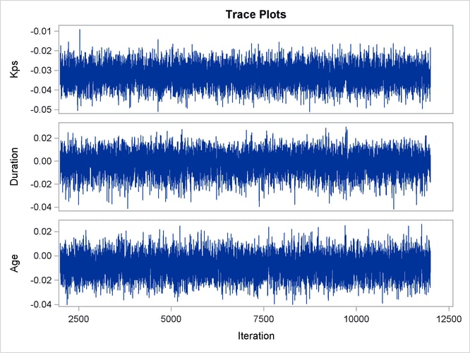
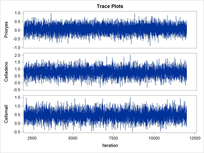
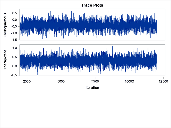
With autocorrelations retreating quickly to 0 (Output 85.13.8) and large effective sample sizes (Output 85.13.9), both diagnostics indicate a reasonably good mixing of the Markov chain. The trace plots in Output 85.13.10 also confirm the convergence of the Markov chain.
Output 85.13.8: Autocorrelation Diagnostics
| Posterior Autocorrelations | ||||
|---|---|---|---|---|
| Parameter | Lag 1 | Lag 5 | Lag 10 | Lag 50 |
| Kps | 0.1442 | -0.0016 | 0.0096 | -0.0013 |
| Duration | 0.2672 | -0.0054 | -0.0004 | -0.0011 |
| Age | 0.1374 | -0.0044 | 0.0129 | 0.0084 |
| Prioryes | 0.2507 | -0.0271 | -0.0012 | 0.0004 |
| Celladeno | 0.4160 | 0.0265 | -0.0062 | 0.0190 |
| Cellsmall | 0.5055 | 0.0277 | -0.0011 | 0.0271 |
| Cellsquamous | 0.3586 | 0.0252 | -0.0044 | 0.0107 |
| Therapytest | 0.2063 | 0.0199 | -0.0047 | -0.0166 |
Output 85.13.9: Effective Sample Size Diagnostics
| Effective Sample Sizes | |||
|---|---|---|---|
| Parameter | ESS | Autocorrelation Time |
Efficiency |
| Kps | 7046.7 | 1.4191 | 0.7047 |
| Duration | 5790.0 | 1.7271 | 0.5790 |
| Age | 7426.1 | 1.3466 | 0.7426 |
| Prioryes | 6102.2 | 1.6388 | 0.6102 |
| Celladeno | 3673.4 | 2.7223 | 0.3673 |
| Cellsmall | 3346.4 | 2.9883 | 0.3346 |
| Cellsquamous | 4052.8 | 2.4674 | 0.4053 |
| Therapytest | 6870.8 | 1.4554 | 0.6871 |
Output 85.13.10: Trace Plots
The first HAZARDRATIO statement compares the hazards between the standard therapy and the test therapy. Summaries of the posterior distribution of the corresponding hazard ratio are shown in Output 85.13.11. There is a 95% chance that the hazard ratio of standard therapy versus test therapy lies between 0.5 and 1.1.
Output 85.13.11: Hazard Ratio for Treatment
The second HAZARDRATIO statement assesses the change of hazards for an increase in Age of 10 years. Summaries of the posterior distribution of the corresponding hazard ratio are shown in Output 85.13.12.
Output 85.13.12: Hazard Ratio for Age
The third HAZARDRATIO statement compares the changes of hazards between two types of cells. For four types of cells, there are six different pairs of cell comparisons. The results are shown in Output 85.13.13.
Output 85.13.13: Hazard Ratios for Cell
| Hazard Ratio Statement 3: Hazard Ratios for cell type | ||||||||||
|---|---|---|---|---|---|---|---|---|---|---|
| Description | N | Mean | Standard Deviation |
Quantiles | ||||||
| 25% | 50% | 75% | 95% Equal-Tail Interval | 95% HPD Interval | ||||||
| Cell adeno vs large | 10000 | 2.3048 | 0.7224 | 1.7929 | 2.1982 | 2.7000 | 1.2067 | 4.0227 | 1.0053 | 3.7057 |
| Cell adeno vs small | 10000 | 1.4377 | 0.4078 | 1.1522 | 1.3841 | 1.6704 | 0.7930 | 2.3999 | 0.7309 | 2.2662 |
| Cell adeno vs squamous | 10000 | 3.4449 | 1.0745 | 2.6789 | 3.2941 | 4.0397 | 1.8067 | 5.9727 | 1.6303 | 5.5946 |
| Cell large vs small | 10000 | 0.6521 | 0.1780 | 0.5264 | 0.6325 | 0.7545 | 0.3618 | 1.0588 | 0.3331 | 1.0041 |
| Cell large vs squamous | 10000 | 1.5579 | 0.4548 | 1.2344 | 1.4955 | 1.8089 | 0.8492 | 2.6346 | 0.7542 | 2.4575 |
| Cell small vs squamous | 10000 | 2.4728 | 0.7081 | 1.9620 | 2.3663 | 2.8684 | 1.3789 | 4.1561 | 1.2787 | 3.9263 |