The PHREG Procedure

Residuals are used to investigate the lack of fit of a model to a given subject. You can obtain martingale and deviance residuals for the Cox proportional hazards regression analysis by requesting that they be included in the OUTPUT data set. You can plot these statistics and look for outliers.

Consider the stepwise regression analysis performed in Example 85.1. The final model included variables LogBUN and HGB. You can generate residual statistics for this analysis by refitting the model containing those variables and including an OUTPUT statement as in the following invocation of PROC PHREG. The keywords XBETA, RESMART, and RESDEV identify new variables that contain the linear predictor scores , martingale residuals, and deviance residuals. These variables are xb, mart, and dev, respectively.

proc phreg data=Myeloma noprint;
   model Time*Vstatus(0)=LogBUN HGB;
   output out=Outp xbeta=Xb resmart=Mart resdev=Dev;
run;

The following statements plot the residuals against the linear predictor scores:

title "Myeloma Study";
proc sgplot data=Outp;
   yaxis grid;
   refline 0 / axis=y;
   scatter y=Mart x=Xb;
run;
proc sgplot data=Outp;
   yaxis grid;
   refline 0 / axis=y;
   scatter y=Dev x=Xb;
run;

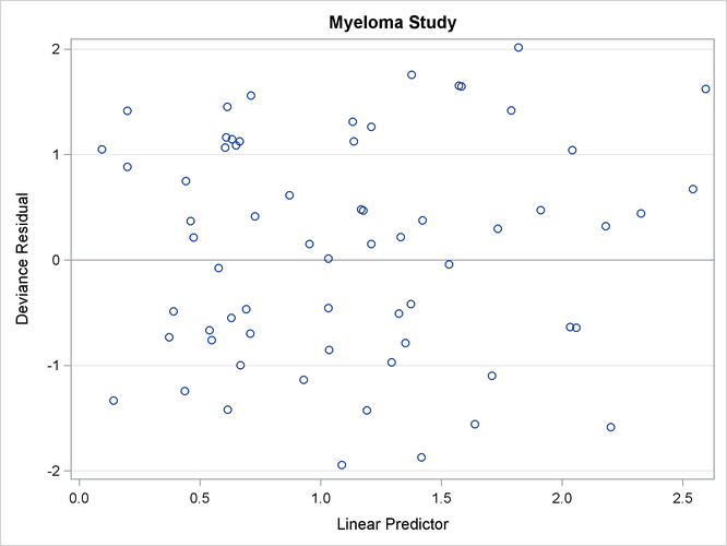
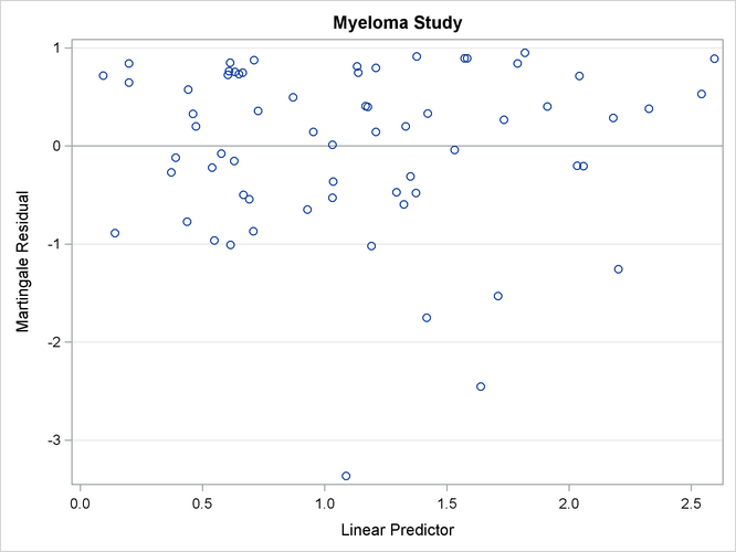
The resulting plots are shown in Output 85.9.1 and Output 85.9.2. The martingale residuals are skewed because of the single event setting of the Cox model. The martingale residual plot shows an isolation point (with linear predictor score 1.09 and martingale residual –3.37), but this observation is no longer distinguishable in the deviance residual plot. In conclusion, there is no indication of a lack of fit of the model to individual observations.