The PHREG Procedure
- Overview
-
Getting Started

-
SyntaxPROC PHREG StatementASSESS StatementBASELINE StatementBAYES StatementBY StatementCLASS StatementCONTRAST StatementEFFECT StatementESTIMATE StatementFREQ StatementHAZARDRATIO StatementID StatementLSMEANS StatementLSMESTIMATE StatementMODEL StatementOUTPUT StatementProgramming StatementsRANDOM StatementSTRATA StatementSLICE StatementSTORE StatementTEST StatementWEIGHT Statement
-
DetailsFailure Time DistributionTime and CLASS Variables UsagePartial Likelihood Function for the Cox ModelCounting Process Style of InputLeft-Truncation of Failure TimesThe Multiplicative Hazards ModelProportional Rates/Means Models for Recurrent EventsThe Frailty ModelProportional Subdistribution Hazards Model for Competing-Risks DataHazard RatiosNewton-Raphson MethodFirth’s Modification for Maximum Likelihood EstimationRobust Sandwich Variance EstimateTesting the Global Null HypothesisType 3 Tests and Joint TestsConfidence Limits for a Hazard RatioUsing the TEST Statement to Test Linear HypothesesAnalysis of Multivariate Failure Time DataModel Fit StatisticsSchemper-Henderson Predictive MeasureResidualsDiagnostics Based on Weighted ResidualsInfluence of Observations on Overall Fit of the ModelSurvivor Function EstimatorsCaution about Using Survival Data with Left TruncationEffect Selection MethodsAssessment of the Proportional Hazards ModelThe Penalized Partial Likelihood Approach for Fitting Frailty ModelsSpecifics for Bayesian AnalysisComputational ResourcesInput and Output Data SetsDisplayed OutputODS Table NamesODS Graphics
-
ExamplesStepwise RegressionBest Subset SelectionModeling with Categorical PredictorsFirth’s Correction for Monotone LikelihoodConditional Logistic Regression for m:n MatchingModel Using Time-Dependent Explanatory VariablesTime-Dependent Repeated Measurements of a CovariateSurvival CurvesAnalysis of ResidualsAnalysis of Recurrent Events DataAnalysis of Clustered DataModel Assessment Using Cumulative Sums of Martingale ResidualsBayesian Analysis of the Cox ModelBayesian Analysis of Piecewise Exponential ModelAnalysis of Competing-Risks Data
- References
Survivor Function Estimators
Three estimators of the survivor function are available: the Breslow (1972) estimator, which is based on the empirical cumulative hazard function, the Fleming and Harrington (1984) estimator, which is a tie-breaking modification of the Breslow estimator, and the product-limit estimator (Kalbfleisch and Prentice 1980, pp. 84–86).
Let  be the distinct uncensored times of the survival data.
Breslow Estimator
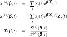
To select this estimator, specify the METHOD=BRESLOW option in the BASELINE statement or OUTPUT statement. For the jth subject, let  represent the failure time, the event indicator, and the vector of covariate values, respectively. For
  , let
, let
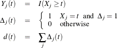
Note that  is the number of subjects that have an event at t. Let
For a given realization of the explanatory variables  , the cumulative hazard function estimator at is
![\[ \hat{\Lambda }_ B(t,\bxi ) = \mr{e}^{\hat{\bbeta }'\bxi } \sum _{t_ i\leq t} \frac{d(t_ i)}{S^{(0)}(\hat{\bbeta },t_ i)} \]](images/statug_phreg0631.png)
with variance estimated by
![\[ \hat{\sigma }^2(\hat{\Lambda }_ B(t,\bxi )) = \mr{e}^{2\hat{\bbeta }'\bxi } \sum _{t_ i \leq t} \frac{d(t_ i)}{[S^{(0)}(\hat{\bbeta },t_ i)]^2} + H(t,\bxi )’[\mc{I}(\hat{\bbeta })]^{-1} H(t,\bxi ) \]](images/statug_phreg0632.png)
where
![\[ H(t,\bxi ) = \mr{e}^{\hat{\bbeta }'\bxi }\sum _{t_ i \leq t} \frac{d(t_ i)}{S^{(0)}(\hat{\bbeta },t_ i)} \biggl ( \bar{\bZ }(\hat{\bbeta },t_ i)- \bxi \biggr ) \]](images/statug_phreg0633.png)
For the marginal model, the variance estimator computation follows Spiekerman and Lin (1998).
The Breslow estimate of the survivor function for  is
is
![\[ \hat{S}_ B(t,\bxi ) = \exp (-\hat{\Lambda }_ B(t,\bxi )) \]](images/statug_phreg0635.png)
By the delta method, the standard error of  is approximated by
![\[ \hat{\sigma }(\hat{S}_ B(t,\bxi )) = \hat{S}_ B(t,\bxi ) \hat{\sigma }(\hat{\Lambda }_ B(t,\bxi )) \]](images/statug_phreg0637.png)
Fleming-Harrington Estimator
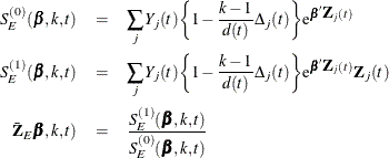
To select this estimator, specify the METHOD=FH option in the BASELINE statement or OUTPUT statement. With  and as defined in the section Breslow Estimator and for
  , let
, let
For a given realization of the explanatory variables, the Fleming-Harrington adjustment of the cumulative hazard function is
![\[ \hat{\Lambda }_ F(t,\bxi ) = \mr{e}^{\hat{\bbeta }'\bxi } \sum _{t_ i\leq t} \biggr \{ \sum _{k=1}^{d(t_ i)} \frac{1}{S_ E^{(0)}(\hat{\bbeta },k,t_ i)} \biggr \} \]](images/statug_phreg0640.png)
with variance estimated by
![\[ \hat{\sigma }^2(\hat{\Lambda }_ F(t,\bxi )) = \mr{e}^{2\hat{\bbeta }'\bxi } \sum _{t_ i \leq t} \biggl \{ \sum _{k=1}^{d(t_ i)} \frac{1}{[S_ E^{(0)}(\hat{\bbeta },k,t_ i)]^2} \biggr \} + H_ E(t,\bxi )’[\mc{I}(\hat{\bbeta })]^{-1} H_ E(t,\bxi ) \]](images/statug_phreg0641.png)
where
![\[ H_ E(t,\bxi ) = \mr{e}^{\hat{\bbeta }'\bxi } \biggl \{ \biggl [\sum _{t_ i \leq t} \sum _{k=1}^{d(t_ i)} \frac{1}{ S_ E^{(0)}(\hat{\bbeta },k,t_ i)} \bar{\bZ }_ E(\hat{\bbeta },k, t_ i) \biggr ] - \hat{\Lambda }_ F(t,\mb{0})\bxi \biggl \} \]](images/statug_phreg0642.png)
The Fleming-Harrington estimate of the survivor function for is
![\[ \hat{S}_ F(t,\bxi ) = \exp (-\hat{\Lambda }_ F(t,\bxi )) \]](images/statug_phreg0643.png)
By the delta method, the standard error of is approximated by
![\[ \hat{\sigma }(\hat{S}_ F(t,\bxi )) = \hat{S}_ F(t,\bxi ) \hat{\sigma }(\hat{\Lambda }_ F(t,\bxi )) \]](images/statug_phreg0644.png)
Product-Limit Estimator
To select this estimator, specify the METHOD=PL option in the BASELINE statement or OUTPUT statement. Let  denote the set of individuals that fail at
  . Let
. Let  denote the set of individuals that are censored in the half-open interval
  , where
  and
and  . Let
. Let  denote the censoring times in , where l ranges over .
The likelihood function for all individuals is given by
![\[ \mc{L}=\prod _{i=0}^{k} \left\{ \prod _{l \in \mc{D}_ i} \left( [S_{0}(t_{i})]^{ \ \mr{exp}(\mb{Z}'_{l}\bbeta ) } -[S_{0}(t_{i}+0)]^{ \ \mr{exp}(\mb{Z}'_{l}\bbeta ) } \right) \prod _{l \in \mc{C}_ i} [S_{0}(\gamma _{l}+0)]^{\ \mr{exp}(\mb{Z}'_{l}\bbeta )} \right\} \]](images/statug_phreg0650.png)
where  is empty. The likelihood
  is maximized by taking
 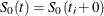 for
for  and allowing the probability mass to fall only on the observed event times
  ,
,  ,
,  . By considering a discrete model with hazard contribution
  at , you take
  , where
  . Substitution into the likelihood function produces
![\[ \mc{L}=\prod _{i=0}^{k} \left\{ \prod _{j \in \mc{D}_ i } \left( 1-\alpha _{i}^{\ \mr{exp}(\mb{Z}'_{j}\bbeta ) } \right) \prod _{ l \in \mc{R}_{i}-\mc{D}_{i} } \alpha _{i}^{ \ \mr{exp}(\mb{z}'_{l}\bbeta )} \right\} \]](images/statug_phreg0661.png)
If you replace  with
with  estimated from the partial likelihood function and then maximize with respect to
  , the maximum likelihood estimate
  of
of  becomes a solution of
![\[ \sum _{ j \in \mc{D}_ i } \frac{ \mr{exp}(\mb{Z}'_{j}\hat{\bbeta }) }{ 1-\hat{\alpha }_{i}^{ \ \mr{exp}(\mb{Z}'_{j}\hat{\bbeta }) } } =\sum _{l \in \mc{R}_ i } \mr{exp}(\mb{Z}’_{l}\hat{\bbeta }) \]](images/statug_phreg0665.png)
When only a single failure occurs at  ,
,  can be found explicitly. Otherwise, an iterative solution is obtained by the Newton method.
The baseline survival function is estimated by
![\[ \hat{S}_{0}(t)=\hat{S}_{0}(t_{i-1}+0) =\prod _{j=0}^{i-1} \hat{\alpha }_{j}, t_{i-1} < t \leq t_{i} \]](images/statug_phreg0668.png)
For a given realization of the explanatory variables , the product-limit estimate of the survival function at is
![\[ \hat{S}_ P(t,\bxi ) = [\hat{S}_{0}(t)]^{\mr{exp}(\bbeta '\bxi )} \]](images/statug_phreg0669.png)
Approximating the variance of  by the variance estimate of the Breslow estimator of the cumulative hazard function, the variance of the product-limit estimator
at is given by
by the variance estimate of the Breslow estimator of the cumulative hazard function, the variance of the product-limit estimator
at is given by
![\[ \hat{\sigma }(\hat{S}_ P(t,\bxi )) = \hat{S}_ P(t,\bxi ) \hat{\sigma }(\hat{\Lambda }_ B(t,\bxi )) \]](images/statug_phreg0671.png)
Direct Adjusted Survival Curves
Consider the Breslow estimator of the survival function. For  , let
, let  represent the covariate set of the jth patient. The direct adjusted survival curve averages the estimated survival curves for each patient:
![\[ \bar{S}(t) = \frac{1}{n}\sum _{j=1}^ n \hat{S}(t,\bxi _ j) \]](images/statug_phreg0674.png)
The variance of  can be estimated by
![\[ \hat{\sigma }^2(\bar{S}(t)) = \frac{1}{n^2} \biggl (V^{(1)}t)+V^{(2)}(t) \biggr ) \]](images/statug_phreg0676.png)
where
![\begin{eqnarray*} V^{(1)}(t)& =& \biggl ( \sum _{j=1}^ n \mr{e}^{\hat{\bbeta }'\bxi _ j} \hat{S}(t,\bxi _ j) \biggr )^2 \sum _{t_ i\leq t} \frac{d(t_ i)}{[S^{(0)}(\hat{\bbeta },t_ i)]^2} \\ V^{(2)}(t)& =& \biggl (\sum _{j=1}^ n \hat{S}(t,\bxi _ j)H(t,\bxi _ j)\biggr )’ \biggl [\mc{I}(\hat{\bbeta }) \biggr ]^{-1} \biggl (\sum _{j=1}^ n \hat{S}(t,\bxi _ j) H(t,\bxi _ j) \biggr ) \end{eqnarray*}](images/statug_phreg0677.png)
Comparison of Direct Adjusted Probabilities of Two Strata
For a stratified Cox model, let k index the strata. For the jth patient, let  and
and  be the estimated survival function and the
  vector for the kth stratum. The direct adjusted survival curve for the kth stratum is
![\[ \bar{S}_ k(t) = \frac{1}{n}\sum _{j=1}^ n \hat{S}_ k(t,\bxi _{j}) \]](images/statug_phreg0681.png)
The variance of  can be estimated by
![\[ \hat{\sigma }^2(\bar{S}_1(t) - \bar{S}_2(t)) = \frac{1}{n^2} \biggl (U^{(1)}_1(t)+U^{(1)}_2 + U^{(2)}_{12}(t) \biggr ) \]](images/statug_phreg0683.png)
where
![\begin{eqnarray*} U^{(1)}_ k(t) & =& \left( \sum _{j=1}^ n \mr{e}^{\bbeta '\bxi _{j}} \hat{S}_ k(t,\bxi _{j}) \right)^2 \sum _{t_ i\leq t} \frac{d(t_ i)}{[S^{(0)}(\hat{\bbeta },t_ i)]^2} \mbox{~ ~ ~ } k=1,2 \\ U^{(2)}_{12}(t)& =& \left\{ \sum _{j=1}^ n \left[\hat{S}_1(t,\bxi _{j})H_1(t,\bxi _{j})-\hat{S}_2(t,\bxi _{j})H_2(t,\bxi _{j}) \right] \right\} ^{\prime } \mc{I} ^{-1}(\hat{\bbeta }) \\ & & \left\{ \sum _{j=1}^ n \left[\hat{S}_1(t,\bxi _{j})H_2(t,\bxi _{j})-\hat{S}_1(t,\bxi _{j})H(_2t,\bxi _{j}) \right] \right\} \end{eqnarray*}](images/statug_phreg0684.png)
Comparison of Direct Adjusted Survival Probabilities of Two Treatments
For , let  represent the covariate set of the jth patient with the kth treatment,
  . The direct adjusted survival curve for the kth treatment is
![\[ \bar{S}_ k(t) = \frac{1}{n}\sum _{i=j}^ n \hat{S}(t,\bxi _{jk}) \]](images/statug_phreg0687.png)
The variance of can be estimated by
![\[ \hat{\sigma }^2\left(\bar{S}_1(t)-\bar{S}_2(t)\right) = \frac{1}{n^2} \biggl (V^{(1)}_{12}(t) + V^{(2)}_{12}(t) \biggr ) \]](images/statug_phreg0688.png)
where
![\begin{eqnarray*} V^{(1)}_{12}(t) & =& \left\{ \sum _{j=1}^ n \left[\mr{e}^{\bbeta '\bxi _{1j}} \hat{S}(t,\bxi _{1j}) - \mr{e}^{\bbeta '\bxi _{2j}} \hat{S}(t,\bxi _{2j}) \right] \right\} ^2 \sum _{t_ i\leq t} \frac{d(t_ i)}{[S^{(0)}(\hat{\bbeta },t_ i)]^2} \\ V^{(2)}_{12}(t)& =& \left\{ \sum _{j=1}^ n \left[\hat{S}(t,\bxi _{1j})H(t,\bxi _{1j})-\hat{S}(t,\bxi _{2j})H(t,\bxi _{2j}) \right] \right\} ^{\prime } \mc{I} ^{-1}(\hat{\bbeta })\\ & & \left\{ \sum _{j=1}^ n \left[\hat{S}(t,\bxi _{1j})H(t,\bxi _{1j})-\hat{S}(t,\bxi _{2j})H(t,\bxi _{2j}) \right] \right\} \end{eqnarray*}](images/statug_phreg0689.png)
Confidence Intervals for the Survivor Function
When the computation of confidence limits for the survivor function  is based on the asymptotic normality of the survival estimator
  —which can be the Breslow estimator
  , the Fleming-Harrington estimator
  , or the product-limit estimator
  —the approximate confidence interval might include impossible values outside the range [0,1] at extreme values of t. This problem can be avoided by applying the asymptotic normality to a transformation of for which the range is unrestricted. In addition, certain transformed confidence intervals for perform better than the usual linear confidence intervals (Borgan and Liestøl 1990). The CLTYPE= option in the BASELINE statement enables you to choose one of the following transformations: the log-log function,
the log function, and the linear function.
—the approximate confidence interval might include impossible values outside the range [0,1] at extreme values of t. This problem can be avoided by applying the asymptotic normality to a transformation of for which the range is unrestricted. In addition, certain transformed confidence intervals for perform better than the usual linear confidence intervals (Borgan and Liestøl 1990). The CLTYPE= option in the BASELINE statement enables you to choose one of the following transformations: the log-log function,
the log function, and the linear function.
Let g be the transformation that is being applied to the survivor function . By the delta method, the standard error of  is estimated by
![\[ \tau (t) = \hat{\sigma }\left[g(\hat{S}(t))\right] = g’\left(\hat{S}(t)\right)\hat{\sigma }[\hat{S}(t)] \]](images/statug_phreg0695.png)
where  is the first derivative of the function g. The 100(1–
 )% confidence interval for is given by
![\[ g^{-1}\left\{ g[\hat{S}(t)] \pm z_{\frac{\alpha }{2}} g’[\hat{S}(t)]\hat{\sigma }[\hat{S}(t)] \right\} \]](images/statug_phreg0697.png)
where  is the inverse function of g. The choices for the transformation g are as follows:
-
CLTYPE=NORMAL specifies linear transformation, which is the same as having no transformation in which g is the identity. The 100(1–
)% confidence interval for is given by
![\[ \hat{S}(t) - z_{\frac{\alpha }{2}}\hat{\sigma }\left[\hat{S}(t)\right] \le S(t) \le \hat{S}(t) + z_{\frac{\alpha }{2}}\hat{\sigma }\left[\hat{S}(t)\right] \]](images/statug_phreg0699.png)
-
CLTYPE=LOG specifies log transformation. The estimated variance of
 is
is  The 100(1–)% confidence interval for is given by
![\[ \hat{S}(t)\exp \left(-z_{\frac{\alpha }{2}}\hat{\tau }(t)\right) \le S(t) \le \hat{S}(t)\exp \left(z_{\frac{\alpha }{2}}\hat{\tau }(t)\right) \]](images/statug_phreg0702.png)
-
CLTYPE=LOGLOG specifies log-log transformation. The estimated variance of
 is
is ![$ \hat{\tau }^2(t) = \frac{\hat{\sigma }^2[\hat{S}(t)]}{ [\hat{S}(t)\log (\hat{S}(t))]^2 }. $](images/statug_phreg0704.png) The 100(1–)% confidence interval for is given by
The 100(1–)% confidence interval for is given by
![\[ \left[\hat{S}(t)\right]^{\exp \left( z_{\frac{\alpha }{2}} \hat{\tau }(t)\right)} \le S(t) \le \left[\hat{S}(t)\right]^{\exp \left(-z_{\frac{\alpha }{2}} \hat{\tau }(t)\right)} \]](images/statug_phreg0705.png)