The PHREG Procedure
- Overview
-
Getting Started

-
SyntaxPROC PHREG StatementASSESS StatementBASELINE StatementBAYES StatementBY StatementCLASS StatementCONTRAST StatementEFFECT StatementESTIMATE StatementFREQ StatementHAZARDRATIO StatementID StatementLSMEANS StatementLSMESTIMATE StatementMODEL StatementOUTPUT StatementProgramming StatementsRANDOM StatementSTRATA StatementSLICE StatementSTORE StatementTEST StatementWEIGHT Statement
-
DetailsFailure Time DistributionTime and CLASS Variables UsagePartial Likelihood Function for the Cox ModelCounting Process Style of InputLeft-Truncation of Failure TimesThe Multiplicative Hazards ModelProportional Rates/Means Models for Recurrent EventsThe Frailty ModelProportional Subdistribution Hazards Model for Competing-Risks DataHazard RatiosNewton-Raphson MethodFirth’s Modification for Maximum Likelihood EstimationRobust Sandwich Variance EstimateTesting the Global Null HypothesisType 3 Tests and Joint TestsConfidence Limits for a Hazard RatioUsing the TEST Statement to Test Linear HypothesesAnalysis of Multivariate Failure Time DataModel Fit StatisticsSchemper-Henderson Predictive MeasureResidualsDiagnostics Based on Weighted ResidualsInfluence of Observations on Overall Fit of the ModelSurvivor Function EstimatorsCaution about Using Survival Data with Left TruncationEffect Selection MethodsAssessment of the Proportional Hazards ModelThe Penalized Partial Likelihood Approach for Fitting Frailty ModelsSpecifics for Bayesian AnalysisComputational ResourcesInput and Output Data SetsDisplayed OutputODS Table NamesODS Graphics
-
ExamplesStepwise RegressionBest Subset SelectionModeling with Categorical PredictorsFirth’s Correction for Monotone LikelihoodConditional Logistic Regression for m:n MatchingModel Using Time-Dependent Explanatory VariablesTime-Dependent Repeated Measurements of a CovariateSurvival CurvesAnalysis of ResidualsAnalysis of Recurrent Events DataAnalysis of Clustered DataModel Assessment Using Cumulative Sums of Martingale ResidualsBayesian Analysis of the Cox ModelBayesian Analysis of Piecewise Exponential ModelAnalysis of Competing-Risks Data
- References
Example 85.15 Analysis of Competing-Risks Data
Bone marrow transplant (BMT) is a standard treatment for acute leukemia. Klein and Moeschberger (1997) present a set of BMT data for 137 patients, grouped into three risk categories based on their status at the time of transplantation: acute lymphoblastic leukemia (ALL), acute myelocytic leukemia (AML) low-risk, and AML high-risk. During the follow-up period, some patients might relapse or some patients might die while in remission. Consider relapse to be the event of interest. Death is a competing risk because death impedes the occurrence of leukemia relapse. The Fine and Gray (1999) model is used to compare the risk categories on the disease-free survival.
The following DATA step creates the data set Bmt. The variable Disease represents the risk group of a patient, which is either ALL, AML-Low Risk, or AML-High Risk. The variable T represents the disease-free survival in days, which is the time to relapse, time to death, or censored. The variable Status has three values: 0 for censored observations, 1 for relapsed patients, and 2 for patients who die before experiencing a
relapse.
proc format;
   value DiseaseGroup 1='ALL'
                      2='AML-Low Risk'
                      3='AML-High Risk';

data Bmt;
   input Disease T Status @@;
   label T='Disease-Free Survival in Days';
   format Disease DiseaseGroup.;
   datalines;
1   2081   0   1   1602   0   1   1496   0   1   1462   0   1   1433   0
1   1377   0   1   1330   0   1    996   0   1    226   0   1   1199   0
1   1111   0   1    530   0   1   1182   0   1   1167   0   1    418   2
1    383   1   1    276   2   1    104   1   1    609   1   1    172   2
1    487   2   1    662   1   1    194   2   1    230   1   1    526   2
1    122   2   1    129   1   1     74   1   1    122   1   1     86   2
1    466   2   1    192   1   1    109   1   1     55   1   1      1   2
1    107   2   1    110   1   1    332   2   2   2569   0   2   2506   0
2   2409   0   2   2218   0   2   1857   0   2   1829   0   2   1562   0
2   1470   0   2   1363   0   2   1030   0   2    860   0   2   1258   0
2   2246   0   2   1870   0   2   1799   0   2   1709   0   2   1674   0
2   1568   0   2   1527   0   2   1324   0   2    957   0   2    932   0
2    847   0   2    848   0   2   1850   0   2   1843   0   2   1535   0
2   1447   0   2   1384   0   2    414   2   2   2204   2   2   1063   2
2    481   2   2    105   2   2    641   2   2    390   2   2    288   2
2    421   1   2     79   2   2    748   1   2    486   1   2     48   2
2    272   1   2   1074   2   2    381   1   2     10   2   2     53   2
2     80   2   2     35   2   2    248   1   2    704   2   2    211   1
2    219   1   2    606   1   3   2640   0   3   2430   0   3   2252   0
3   2140   0   3   2133   0   3   1238   0   3   1631   0   3   2024   0
3   1345   0   3   1136   0   3    845   0   3    422   1   3    162   2
3     84   1   3    100   1   3      2   2   3     47   1   3    242   1
3    456   1   3    268   1   3    318   2   3     32   1   3    467   1
3     47   1   3    390   1   3    183   2   3    105   2   3    115   1
3    164   2   3     93   1   3    120   1   3     80   2   3    677   2
3     64   1   3    168   2   3     74   2   3     16   2   3    157   1
3    625   1   3     48   1   3    273   1   3     63   2   3     76   1
3    113   1   3    363   2
;
PROC PHREG enables you to plot the cumulative incidence function for each disease category, but first you must save these
three Disease values in a SAS data set, as in the following DATA step:
data Risk;
   Disease=1; output;
   Disease=2; output;
   Disease=3; output;
   format Disease DiseaseGroup.;
   run;
The following statements use the PHREG procedure to fit the proportional subdistribution hazards model. To designate relapse (Status=1) as the event of interest, you specify EVENTCODE=1 in the MODEL statement. The HAZARDRATIO statement provides the hazard ratios for all pairs of disease groups. The COVARIATES= option in the BASELINE statement specifies the data set that contains the covariate settings for predicting cumulative incidence functions; and the OUT= option saves the prediction results in a SAS data set. The PLOTS= option in the PROC PHREG statement displays the cumulative incidence curves.
ods graphics on;
proc phreg data=Bmt plots(overlay=stratum)=cif;
   class Disease (order=internal ref=first);
   model T*Status(0)=Disease / eventcode=1;
   Hazardratio 'Pairwise' Disease / diff=pairwise;
   baseline covariates=Risk out=out1 cif=_all_ / seed=191;
run;
Output 85.15.1 displays the codes of different types of observations in the input data set. Relapse is the failure of interest with Status = 1, death is a competing failure with Status = 2, and censored observations are those with Status = 0. Out of the 137 transplant patients, 42 have a relapse, 41 die without experiencing a relapse, and 54 are censored (Output 85.15.2).
Output 85.15.1: Code for the Competing Failures and Censored Observations
Output 85.15.2: Distribution of Events and Censored Observations
Output 85.15.3 shows a significant effect (p = 0.0030) of Disease on the disease-free survival. With the reference coding, the CLASS variable Disease is represented by two dummy variables. Parameter estimates and Wald tests for individual parameters are shown in Output 85.15.3.
Output 85.15.3: Wald Test of the Disease Effect
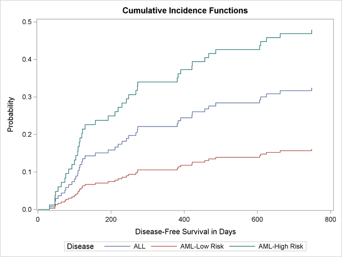
Hazard ratio estimates of one disease group relative to another disease group are displayed in Output 85.15.4. The hazard of relapse for the ALL patients is 2.2 times that for the AML-low risk patients, and the hazard for the AML-high risk patients is 1.7 times that for the ALL patients. It is expected that at any given time after the transplant, an AML high-risk patient is more likely to relapse than an ALL patient, and an ALL patient is more likely to relapse than an AML low-risk patient. Such ordering of probabilities is revealed in the plot of the cumulative incidence functions in Output 85.15.5.
Output 85.15.4: Pairwise Comparison of Disease Group
| Pairwise: Hazard Ratios for Disease | |||
|---|---|---|---|
| Description | Point Estimate | 95% Wald Confidence Limits | |
| Disease ALL vs AML-Low Risk | 2.233 | 0.964 | 5.171 |
| Disease AML-Low Risk vs ALL | 0.448 | 0.193 | 1.037 |
| Disease ALL vs AML-High Risk | 0.601 | 0.293 | 1.233 |
| Disease AML-High Risk vs ALL | 1.663 | 0.811 | 3.408 |
| Disease AML-Low Risk vs AML-High Risk | 0.269 | 0.127 | 0.573 |
| Disease AML-High Risk vs AML-Low Risk | 3.713 | 1.745 | 7.900 |
Output 85.15.5: CIF of the Three Disease Groups
You use the following statements to display the cumulative incidence prediction for the ALL (Disease=1) risk group:
proc print data=Out1(where=(Disease=1));
   title 'CIF Estimates and 95% Confidence limits for the ALL Group';
run;
Output 85.15.6: Cumulative Incidence Prediction
| CIF Estimates and 95% Confidence limits for the ALL Group |
| Obs | Disease | T | CIF | StdErrCIF | LowerCIF | UpperCIF |
|---|---|---|---|---|---|---|
| 1 | ALL | 0 | 0.00000 | . | . | . |
| 2 | ALL | 32 | 0.00727 | 0.007237 | 0.00103 | 0.05114 |
| 3 | ALL | 47 | 0.02183 | 0.014323 | 0.00604 | 0.07898 |
| 4 | ALL | 48 | 0.02922 | 0.017822 | 0.00884 | 0.09657 |
| 5 | ALL | 55 | 0.03663 | 0.019106 | 0.01318 | 0.10181 |
| 6 | ALL | 64 | 0.04405 | 0.019259 | 0.01870 | 0.10378 |
| 7 | ALL | 74 | 0.05151 | 0.019951 | 0.02411 | 0.11005 |
| 8 | ALL | 76 | 0.05897 | 0.025533 | 0.02524 | 0.13778 |
| 9 | ALL | 84 | 0.06646 | 0.025378 | 0.03145 | 0.14048 |
| 10 | ALL | 93 | 0.07400 | 0.025092 | 0.03807 | 0.14383 |
| 11 | ALL | 100 | 0.08158 | 0.030460 | 0.03924 | 0.16959 |
| 12 | ALL | 104 | 0.08920 | 0.029038 | 0.04712 | 0.16883 |
| 13 | ALL | 109 | 0.09682 | 0.033564 | 0.04907 | 0.19100 |
| 14 | ALL | 110 | 0.10443 | 0.035734 | 0.05341 | 0.20422 |
| 15 | ALL | 113 | 0.11205 | 0.041176 | 0.05453 | 0.23026 |
| 16 | ALL | 115 | 0.11972 | 0.037619 | 0.06467 | 0.22163 |
| 17 | ALL | 120 | 0.12742 | 0.036521 | 0.07266 | 0.22347 |
| 18 | ALL | 122 | 0.13518 | 0.042929 | 0.07254 | 0.25190 |
| 19 | ALL | 129 | 0.14293 | 0.041747 | 0.08063 | 0.25336 |
| 20 | ALL | 157 | 0.15068 | 0.046376 | 0.08243 | 0.27545 |
| 21 | ALL | 192 | 0.15848 | 0.051406 | 0.08392 | 0.29928 |
| 22 | ALL | 211 | 0.16628 | 0.058106 | 0.08383 | 0.32983 |
| 23 | ALL | 219 | 0.17404 | 0.056257 | 0.09236 | 0.32794 |
| 24 | ALL | 230 | 0.18185 | 0.053563 | 0.10210 | 0.32392 |
| 25 | ALL | 242 | 0.18967 | 0.065355 | 0.09653 | 0.37265 |
| 26 | ALL | 248 | 0.19753 | 0.057829 | 0.11128 | 0.35062 |
| 27 | ALL | 268 | 0.20535 | 0.054765 | 0.12176 | 0.34634 |
| 28 | ALL | 272 | 0.21322 | 0.058189 | 0.12489 | 0.36402 |
| 29 | ALL | 273 | 0.22105 | 0.061340 | 0.12832 | 0.38080 |
| 30 | ALL | 381 | 0.22893 | 0.061228 | 0.13554 | 0.38669 |
| 31 | ALL | 383 | 0.23677 | 0.062212 | 0.14147 | 0.39626 |
| 32 | ALL | 390 | 0.24461 | 0.063708 | 0.14682 | 0.40754 |
| 33 | ALL | 421 | 0.25250 | 0.070833 | 0.14571 | 0.43757 |
| 34 | ALL | 422 | 0.26035 | 0.063694 | 0.16118 | 0.42053 |
| 35 | ALL | 456 | 0.26825 | 0.067518 | 0.16379 | 0.43932 |
| 36 | ALL | 467 | 0.27621 | 0.073253 | 0.16424 | 0.46450 |
| 37 | ALL | 486 | 0.28422 | 0.066216 | 0.18004 | 0.44871 |
| 38 | ALL | 606 | 0.29233 | 0.067521 | 0.18590 | 0.45971 |
| 39 | ALL | 609 | 0.30039 | 0.079301 | 0.17905 | 0.50396 |
| 40 | ALL | 625 | 0.30845 | 0.067182 | 0.20128 | 0.47270 |
| 41 | ALL | 662 | 0.31657 | 0.070668 | 0.20439 | 0.49033 |
| 42 | ALL | 748 | 0.32469 | 0.082845 | 0.19692 | 0.53537 |
Output 85.15.6 shows the point estimate and the confidence limits for the cumulative incidence at each distinct time when the event of interest occurred for the ALL patients. The predictions for the AML-low risk patients and AML-high risk patients are not shown.