The PHREG Procedure
- Overview
-
Getting Started

-
SyntaxPROC PHREG StatementASSESS StatementBASELINE StatementBAYES StatementBY StatementCLASS StatementCONTRAST StatementEFFECT StatementESTIMATE StatementFREQ StatementHAZARDRATIO StatementID StatementLSMEANS StatementLSMESTIMATE StatementMODEL StatementOUTPUT StatementProgramming StatementsRANDOM StatementSTRATA StatementSLICE StatementSTORE StatementTEST StatementWEIGHT Statement
-
DetailsFailure Time DistributionTime and CLASS Variables UsagePartial Likelihood Function for the Cox ModelCounting Process Style of InputLeft-Truncation of Failure TimesThe Multiplicative Hazards ModelProportional Rates/Means Models for Recurrent EventsThe Frailty ModelProportional Subdistribution Hazards Model for Competing-Risks DataHazard RatiosNewton-Raphson MethodFirth’s Modification for Maximum Likelihood EstimationRobust Sandwich Variance EstimateTesting the Global Null HypothesisType 3 Tests and Joint TestsConfidence Limits for a Hazard RatioUsing the TEST Statement to Test Linear HypothesesAnalysis of Multivariate Failure Time DataModel Fit StatisticsSchemper-Henderson Predictive MeasureResidualsDiagnostics Based on Weighted ResidualsInfluence of Observations on Overall Fit of the ModelSurvivor Function EstimatorsCaution about Using Survival Data with Left TruncationEffect Selection MethodsAssessment of the Proportional Hazards ModelThe Penalized Partial Likelihood Approach for Fitting Frailty ModelsSpecifics for Bayesian AnalysisComputational ResourcesInput and Output Data SetsDisplayed OutputODS Table NamesODS Graphics
-
ExamplesStepwise RegressionBest Subset SelectionModeling with Categorical PredictorsFirth’s Correction for Monotone LikelihoodConditional Logistic Regression for m:n MatchingModel Using Time-Dependent Explanatory VariablesTime-Dependent Repeated Measurements of a CovariateSurvival CurvesAnalysis of ResidualsAnalysis of Recurrent Events DataAnalysis of Clustered DataModel Assessment Using Cumulative Sums of Martingale ResidualsBayesian Analysis of the Cox ModelBayesian Analysis of Piecewise Exponential ModelAnalysis of Competing-Risks Data
- References
Residuals
This section describes the computation of residuals (RESMART=, RESDEV=, RESSCH=, and RESSCO=) in the OUTPUT statement.
First, consider TIES=BRESLOW. Let
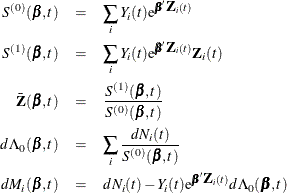
The martingale residual at t is defined as
![\[ \hat{M}_ i(t) = \int _0^ t dM_ i(\hat{\bbeta },s) = N_ i(t) - \int _0^ t Y_ i(s) \mr{e}^{\hat{\bbeta }'\bZ _ i(s)} d\Lambda _0(\hat{\bbeta },s) \]](images/statug_phreg0578.png)
Here  estimates the difference over
 ![$(0,t]$](images/statug_phreg0221.png) between the observed number of events for the ith subject and a conditional expected number of events. The quantity
between the observed number of events for the ith subject and a conditional expected number of events. The quantity  is referred to as the martingale residual for the ith subject. When the counting process MODEL specification is used, the RESMART= variable contains the component (
 ) instead of the martingale residual at
  . The martingale residual for a subject can be obtained by summing up these component residuals within the subject. For the
Cox model with no time-dependent explanatory variables, the martingale residual for the ith subject with observation time
. The martingale residual for a subject can be obtained by summing up these component residuals within the subject. For the
Cox model with no time-dependent explanatory variables, the martingale residual for the ith subject with observation time  and event status
  is
is
![\[ \hat{M}_ i = \Delta _ i - \mr{e}^{\hat{\bbeta }'\bZ _ i} \int _0^{t_ i}d\Lambda _0(\hat{\bbeta },s) \]](images/statug_phreg0582.png)
The deviance residuals  are a transform of the martingale residuals:
![\[ D_{i}= \mr{sign}(\hat{M}_ i)\sqrt {2 \biggl [ -\hat{M}_ i - N_{i}(\infty ) \log \biggl ( \frac{N_{i}(\infty ) - \hat{M}_ i}{N_{i}(\infty )} \biggr ) \biggr ]} \]](images/statug_phreg0584.png)
The square root shrinks large negative martingale residuals, while the logarithmic transformation expands martingale residuals that are close to unity. As such, the deviance residuals are more symmetrically distributed around zero than the martingale residuals. For the Cox model, the deviance residual reduces to the form
![\[ D_{i}= \mr{sign}(\hat{M}_ i)\sqrt {2 [ -\hat{M}_ i - \Delta _ i \log ( \Delta _ i - \hat{M}_ i)]} \]](images/statug_phreg0585.png)
When the counting process MODEL specification is used, values of the RESDEV= variable are set to missing because the deviance residuals can be calculated only on a per-subject basis.
The Schoenfeld (1982) residual vector
is calculated on a per-event-time basis. At the jth event time  of the ith subject, the Schoenfeld residual
![\[ \hat{\bU }_{i}(t_{i_ j}) = \bZ _{i}(t_{i_ j}) - \bar{\bZ }(\hat{\bbeta },t_{i_ j}) \]](images/statug_phreg0587.png)
is the difference between the ith subject covariate vector at and the average of the covariate vectors over the risk set at . Under the proportional hazards assumption, the Schoenfeld residuals have the sample path of a random walk; therefore, they
are useful in assessing time trend or lack of proportionality. Harrell (1986) proposed a z-transform of the Pearson correlation between these residuals and the rank order of the failure time as a test statistic for
nonproportional hazards. Therneau, Grambsch, and Fleming (1990) considered a Kolmogorov-type test based on the cumulative sum of the residuals.
The score process for the ith subject at time t is
![\[ \bL _{i}(\bbeta ,t) = \int _{0}^{t} [\bZ _{i}(s) - \bar{\bZ }(\bbeta ,s)] dM_{i}(\bbeta , s) \]](images/statug_phreg0588.png)
The vector  is the score residual for the ith subject. When the counting process MODEL specification is used, the RESSCO= variables contain the components of
 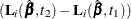 instead of the score process at . The score residual for a subject can be obtained by summing up these component residuals within the subject.
The score residuals are a decomposition of the first partial derivative of the log likelihood. They are useful in assessing the influence of each subject on individual parameter estimates. They also play an important role in the computation of the robust sandwich variance estimators of Lin and Wei (1989) and Wei, Lin, and Weissfeld (1989).
For TIES=EFRON, the preceding computation is modified to comply with the Efron partial likelihood. For a given time t, let  =1 if the t is an event time of the ith subject and 0 otherwise. Let
  , which is the number of subjects that have an event at t. For
  , let
, let
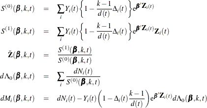
The martingale residual at t for the ith subject is defined as
![\[ \hat{M}_ i(t) = \int _0^ t \frac{1}{d(s)} \sum _{k=1}^{d(s)} dM_ i(\hat{\bbeta },k,s) = N_ i(t) - \int _0^ t \frac{1}{d(s)} \sum _{k=1}^{d(s)} Y_ i(s)\biggl ( 1- \Delta _ i(s) \frac{k-1}{d(s)} \biggr ) \mr{e}^{\hat{\bbeta }'\bZ _ i(s)} d\Lambda _0(\hat{\bbeta },k,s) \]](images/statug_phreg0595.png)
Deviance residuals are computed by using the same transform on the corresponding martingale residuals as in TIES=BRESLOW.
The Schoenfeld residual vector
for the ith subject at event time is
![\[ \hat{\bU }_{i}(t_{i_ j}) = \bZ _{i}(t_{i_ j}) - \frac{1}{d(t_{i_ j})}\sum _{k=1}^{d(t_{i_ j})}\bar{\bZ }(\hat{\bbeta },k,t_{i_ j}) \]](images/statug_phreg0596.png)
The score process for the ith subject at time t is given by
![\[ \bL _{i}(\bbeta ,t) = \int _0^ t \frac{1}{d(s)} \sum _{k=1}^{d(s)}\biggl (\bZ _{i}(s) - \bar{\bZ }(\bbeta ,k,s) \biggr ) dM_{i}(\bbeta ,k,s) \\ \]](images/statug_phreg0597.png)
For TIES=DISCRETE or TIES=EXACT, it is difficult to come up with modifications that are consistent with the corresponding partial likelihood. Residuals for these TIES= methods are computed by using the same formulas as in TIES=BRESLOW.