The PHREG Procedure
- Overview
-
Getting Started

-
SyntaxPROC PHREG StatementASSESS StatementBASELINE StatementBAYES StatementBY StatementCLASS StatementCONTRAST StatementEFFECT StatementESTIMATE StatementFREQ StatementHAZARDRATIO StatementID StatementLSMEANS StatementLSMESTIMATE StatementMODEL StatementOUTPUT StatementProgramming StatementsRANDOM StatementSTRATA StatementSLICE StatementSTORE StatementTEST StatementWEIGHT Statement
-
DetailsFailure Time DistributionTime and CLASS Variables UsagePartial Likelihood Function for the Cox ModelCounting Process Style of InputLeft-Truncation of Failure TimesThe Multiplicative Hazards ModelProportional Rates/Means Models for Recurrent EventsThe Frailty ModelProportional Subdistribution Hazards Model for Competing-Risks DataHazard RatiosNewton-Raphson MethodFirth’s Modification for Maximum Likelihood EstimationRobust Sandwich Variance EstimateTesting the Global Null HypothesisType 3 Tests and Joint TestsConfidence Limits for a Hazard RatioUsing the TEST Statement to Test Linear HypothesesAnalysis of Multivariate Failure Time DataModel Fit StatisticsSchemper-Henderson Predictive MeasureResidualsDiagnostics Based on Weighted ResidualsInfluence of Observations on Overall Fit of the ModelSurvivor Function EstimatorsCaution about Using Survival Data with Left TruncationEffect Selection MethodsAssessment of the Proportional Hazards ModelThe Penalized Partial Likelihood Approach for Fitting Frailty ModelsSpecifics for Bayesian AnalysisComputational ResourcesInput and Output Data SetsDisplayed OutputODS Table NamesODS Graphics
-
ExamplesStepwise RegressionBest Subset SelectionModeling with Categorical PredictorsFirth’s Correction for Monotone LikelihoodConditional Logistic Regression for m:n MatchingModel Using Time-Dependent Explanatory VariablesTime-Dependent Repeated Measurements of a CovariateSurvival CurvesAnalysis of ResidualsAnalysis of Recurrent Events DataAnalysis of Clustered DataModel Assessment Using Cumulative Sums of Martingale ResidualsBayesian Analysis of the Cox ModelBayesian Analysis of Piecewise Exponential ModelAnalysis of Competing-Risks Data
- References
Analysis of Multivariate Failure Time Data
Multivariate failure time data arise when each study subject can potentially experience several events (for instance, multiple infections after surgery) or when there exists some natural or artificial clustering of subjects (for instance, a litter of mice) that induces dependence among the failure times of the same cluster. Data in the former situation are referred to as multiple events data, and data in the latter situation are referred to as clustered data. The multiple events data can be further classified into ordered and unordered data. For ordered data, there is a natural ordering of the multiple failures within a subject, which includes recurrent events data as a special case. For unordered data, the multiple event times result from several concurrent failure processes.
Multiple events data can be analyzed by the Wei, Lin, and Weissfeld (1989), or WLW, method based on the marginal Cox models. For the special case of recurrent events data, you can fit the intensity model (Andersen and Gill 1982), the proportional rates/means model (Pepe and Cai 1993; Lawless and Nadeau 1995; Lin et al. 2000), or the stratified models for total time and gap time proposed by Prentice, Williams, and Peterson (1981), or PWP. For clustered data, you can carry out the analysis of Lee, Wei, and Amato (1992) based on the marginal Cox model. To use PROC PHREG to perform these analyses correctly and effectively, you have to array your data in a specific way to produce the correct risk sets.
All examples described in this section can be found in the program phrmult.sas in the SAS/STAT sample library. Furthermore, the "Examples" section in this chapter contains two examples to illustrate the methods of analyzing recurrent events data and clustered data.
Marginal Cox Models for Multiple Events Data
Suppose there are n subjects and each subject can experience up to K potential events. Let  be the covariate process associated with the kth event for the ith subject. The marginal Cox models are given by
![\[ \lambda _ k(t;\bZ _{ki}) = \lambda _{k0} \mr{e}^{\bbeta _ k'\bZ _{ki}(t)}, k=1,\ldots , K; i=1,\ldots ,n \]](images/statug_phreg0514.png)
where  is the (event-specific) baseline hazard function for the kth event and
  is the (event-specific) column vector of regression coefficients for the kth event. WLW
estimates
is the (event-specific) column vector of regression coefficients for the kth event. WLW
estimates  by the maximum partial likelihood estimates
  , respectively, and uses a robust sandwich covariance matrix estimate for
  to account for the dependence of the multiple failure times.
By using a properly prepared input data set, you can estimate the regression parameters for all the marginal Cox models and
compute the robust sandwich covariance estimates in one PROC PHREG invocation. For convenience of discussion, suppose each
subject can potentially experience K = 3 events and there are two explanatory variables Z1 and Z2. The event-specific parameters to be estimated are  for the first marginal model,
  for the second marginal model, and
  for the third marginal model. Inference of these parameters is based on the robust sandwich covariance matrix estimate of
the parameter estimators. It is necessary that each row of the input data set represent the data for a potential event of
a subject. The input data set should contain the following:
for the third marginal model. Inference of these parameters is based on the robust sandwich covariance matrix estimate of
the parameter estimators. It is necessary that each row of the input data set represent the data for a potential event of
a subject. The input data set should contain the following:
-
an
IDvariable for identifying the subject so that all observations of the same subject have the sameIDvalue -
an
Enumvariable to index the multiple events. For example,Enum=1 for the first event,Enum=2 for the second event, and so on. -
a
Timevariable to represent the observed time from some time origin for the event. For recurrence events data, it is the time from the study entry to each recurrence. -
a
Statusvariable to indicate whether theTimevalue is a censored or uncensored time. For example, Status=1 indicates an uncensored time and Status=0 indicates a censored time. -
independent variables (
Z1andZ2)
The WLW analysis can be carried out by specifying the following:
proc phreg covs(aggregate);
   model Time*Status(0)=Z11 Z12 Z13 Z21 Z22 Z23;
   strata Enum;
   id ID;
   Z11= Z1 * (Enum=1);
   Z12= Z1 * (Enum=2);
   Z13= Z1 * (Enum=3);
   Z21= Z2 * (Enum=1);
   Z22= Z2 * (Enum=2);
   Z23= Z2 * (Enum=3);
run;
The variable Enum is specified in the STRATA statement so that there is one marginal Cox model for each distinct value of Enum. The variables Z11, Z12, Z13, Z21, Z22, and Z23 in the MODEL statement are event-specific variables derived from the independent variables Z1 and Z2 by the given programming statements. In particular, the variables Z11, Z12, and Z13 are event-specific variables for the explanatory variable Z1; the variables Z21, Z22, and Z23 are event-specific variables for the explanatory variable Z2. For  , and
, and  , variable
 Zjk contains the same values as the explanatory variable Zj for the rows that correspond to kth marginal model and the value 0 for all other rows; as such,  is the regression coefficient for
 Zjk. You can avoid using the programming statements in PROC PHREG if you create these event-specific variables in the input data
set by using the same programming statements in a DATA step.
The option COVS(AGGREGATE) is specified in the PROC PHREG statement to obtain the robust sandwich estimate of the covariance matrix, and the score residuals used in computing the middle part of the sandwich estimate are aggregated over identical ID values. You can also include TEST statements in the PROC PHREG code to test various linear hypotheses of the regression parameters based on the robust sandwich covariance matrix estimate.
Consider the AIDS study data in Wei, Lin, and Weissfeld (1989) from a randomized clinical trial to assess the antiretroviral capacity of ribavirin over time in AIDS patients. Blood samples were collected at weeks 4, 8, and 12 from each patient in three treatment groups (placebo, low dose of ribavirin, and high dose). For each serum sample, the failure time is the number of days before virus positivity was detected. If the sample was contaminated or it took a longer period of time than was achievable in the laboratory, the sample was censored. For example:
-
Patient #1 in the placebo group has uncensored times 9, 6, and 7 days (that is, it took 9 days to detect viral positivity in the first blood sample, 6 days for the second blood sample, and 7 days for the third blood sample).
-
Patient #14 in the low-dose group of ribavirin has uncensored times of 16 and 17 days for the first and second sample, respectively, and a censored time of 21 days for the third blood sample.
-
Patient #28 in the high-dose group has an uncensored time of 21 days for the first sample, no measurement for the second blood sample, and a censored time of 25 days for the third sample.
For a full-rank parameterization, two design variables are sufficient to represent three treatment groups. Based on the reference coding with placebo as the reference, the values of the two dummy explanatory variables Z1 and Z2 representing the treatments are as follows:
|
Treatment Group |
|
|
|---|---|---|
|
Placebo |
0 |
0 |
|
Low dose ribavirin |
1 |
0 |
|
High dose ribavirin |
0 |
1 |
The bulk of the task in using PROC PHREG to perform the WLW analysis lies in the preparation of the input data set. As discussed
earlier, the input data set should contain the ID, Enum, Time, and Status variables, and event-specific independent variables Z11, Z12, Z13, Z21, Z22, and Z23. Data for the three patients described
earlier are arrayed as follows:
|
|
|
|
|
|
|
|---|---|---|---|---|---|
|
1 |
9 |
1 |
1 |
0 |
0 |
|
1 |
6 |
1 |
2 |
0 |
0 |
|
1 |
7 |
1 |
3 |
0 |
0 |
|
14 |
16 |
1 |
1 |
1 |
0 |
|
14 |
17 |
1 |
2 |
1 |
0 |
|
14 |
21 |
0 |
3 |
1 |
0 |
|
28 |
21 |
1 |
1 |
0 |
1 |
|
28 |
25 |
0 |
3 |
0 |
1 |
The first three rows are data for Patient #1 with event times at 9, 6, and 7 days, one row for each event. The next three
rows are data for Patient #14, who has an uncensored time of 16 days for the first serum sample, an uncensored time of 17
days for the second sample, and a censored time of 21 days for the third sample. The last two rows are data for Patient #28
of the high-dose group (Z1=0 and Z2=1). Since the patient did not have a second serum sample, there are only two rows of data.
To perform the WLW analysis, you specify the following statements:
proc phreg covs(aggregate);
   model Time*Status(0)=Z11 Z12 Z13 Z21 Z22 Z23;
   strata Enum;
   id ID;
   Z11= Z1 * (Enum=1);
   Z12= Z1 * (Enum=2);
   Z13= Z1 * (Enum=3);
   Z21= Z2 * (Enum=1);
   Z22= Z2 * (Enum=2);
   Z23= Z2 * (Enum=3);
   EqualLowDose: test Z11=Z12, Z12=Z23;
   AverageLow: test Z11,Z12,Z13 / e average;
run;
Two linear hypotheses are tested using the TEST statements. The specification
EqualLowDose: test Z11=Z12, Z12=Z13;
tests the null hypothesis  of identical low-dose effects across three marginal models. The specification
AverageLow: test Z11,Z12,Z13 / e average;
tests the null hypothesis of no low-dose effects (that is, 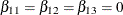 ). The AVERAGE option computes the optimal weights for estimating the average low-dose effect
 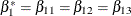 and performs a 1 DF test for testing the null hypothesis that
  . The E option displays the coefficients for the linear hypotheses, including the optimal weights.
Marginal Cox Models for Clustered Data
Suppose there are n clusters with  members in the ith cluster,
  . Let be the covariate process associated with the kth member of the ith cluster. The marginal Cox model is given by
![\[ \lambda (t;\bZ _{ki}) = \lambda _{0}(t) \mr{e}^{\bbeta '\bZ _{ki}(t)} k=1,\ldots , K_ i; i=1,\ldots ,n \]](images/statug_phreg0531.png)
where  is an arbitrary baseline hazard function and
  is the vector of regression coefficients. Lee, Wei, and Amato (1992)
estimate by the maximum partial likelihood estimate
is the vector of regression coefficients. Lee, Wei, and Amato (1992)
estimate by the maximum partial likelihood estimate  under the independent working assumption, and use a robust sandwich covariance estimate to account for the intracluster dependence.
To use PROC PHREG to analyze the clustered data, each member of a cluster is represented by an observation in the input data set. The input data set to PROC PHREG should contain the following:
-
an
IDvariable to identify the cluster so that members of the same cluster have the same ID value -
a
Timevariable to represent the observed survival time of a member of a cluster -
a
Statusvariable to indicate whether the Time value is an uncensored or censored time. For example, Status=1 indicates an uncensored time and Status=0 indicates a censored time. -
the explanatory variables thought to be related to the failure time
Consider a tumor study in which one of three female rats of the same litter was randomly subjected to a drug treatment. The failure time is the time from randomization to the detection of tumor. If a rat died before the tumor was detected, the failure time was censored. For example:
-
In litter #1, the drug-treated rat has an uncensored time of 101 days, one untreated rat has a censored time of 49 days, and the other untreated rat has a failure time of 104 days.
-
In litter #3, the drug-treated rat has a censored time of 104 days, one untreated rat has a censored time of 102 days, and the other untreated rat has a censored time of 104 days.
In this example, a litter is a cluster and the rats of the same litter are members of the cluster. Let Trt be a 0-1 variable representing the treatment a rat received, with value 1 for drug treatment and 0 otherwise. Data for the
two litters of rats described earlier contribute six observations to the input data set:
|
|
|
|
|
|---|---|---|---|
|
1 |
101 |
1 |
1 |
|
1 |
49 |
0 |
0 |
|
1 |
104 |
1 |
0 |
|
3 |
104 |
0 |
1 |
|
3 |
102 |
0 |
0 |
|
3 |
104 |
0 |
0 |
The analysis of Lee, Wei, and Amato (1992) can be performed by PROC PHREG as follows:
proc phreg covs(aggregate);
   model Time*Status(0)=Treatment;
   id Litter;
run;
Intensity and Rate/Mean Models for Recurrent Events Data
Suppose each subject experiences recurrences of the same phenomenon. Let  be the number of events a subject experiences over the interval [0,t] and let
  be the covariate process of the subject.
The intensity model (Andersen and Gill 1982) is given by
![\[ \lambda _{\bZ }(t)dt = E\{ dN(t)|\mc{F}_{t-}\} =\lambda _0(t)\mr{e}^{\bbeta '\bZ (t)}dt \]](images/statug_phreg0533.png)
where  represents all the information of the processes N and
  up to time t, is an arbitrary baseline intensity function, and is the vector of regression coefficients. This model consists of two components: (1) all the influence of the prior events
on future recurrences, if there is any, is mediated through the time-dependent covariates, and (2) the covariates have multiplicative
effects on the instantaneous rate of the counting process. If the covariates are time invariant, the risk of recurrences is
unaffected by the past events.
up to time t, is an arbitrary baseline intensity function, and is the vector of regression coefficients. This model consists of two components: (1) all the influence of the prior events
on future recurrences, if there is any, is mediated through the time-dependent covariates, and (2) the covariates have multiplicative
effects on the instantaneous rate of the counting process. If the covariates are time invariant, the risk of recurrences is
unaffected by the past events.
The proportional rates and means models (Pepe and Cai 1993; Lawless and Nadeau 1995; Lin et al. 2000) assume that the covariates have multiplicative effects on the mean and rate functions of the counting process. The rate function is given by
![\[ d\mu _{\bZ }(t)= E\{ dN(t)|\bZ (t)\} =\mr{e}^{\bbeta '\bZ (t)} d\mu _{0}(t) \]](images/statug_phreg0535.png)
where  is an unknown continuous function and is the vector of regression parameters. If is time invariant, the mean function
is given by
is an unknown continuous function and is the vector of regression parameters. If is time invariant, the mean function
is given by
![\[ \mu _{\bZ }(t) = E\{ N(t) | \bZ \} = \mr{e}^{\bbeta '\bZ }\mu _0(t) \]](images/statug_phreg0537.png)
For both the intensity and the proportional rates/means models, estimates of the regression coefficients are obtained by solving the partial likelihood score function. However, the covariance matrix estimate for the intensity model is computed as the inverse of the observed information matrix, while that for the proportional rates/means model is given by a sandwich estimate. For a given pattern of fixed covariates, the Nelson estimate for the cumulative intensity function is the same for the cumulative mean function, but their standard errors are not the same.
To fit the intensity or rate/mean model by using PROC PHREG, the counting process style of input is needed. A subject with
K events contributes K + 1 observations to the input data set. The kth observation of the subject identifies the time interval from the (k – 1) event or time 0 (if k = 1) to the kth event,  . The (K + 1) observation represents the time interval from the Kth event to time of censorship. The input data set should contain the following variables:
-
a
TStartvariable to represent the (k – 1) recurrence time or the value 0 if k = 1 -
a
TStopvariable to represent the kth recurrence time or the follow-up time if k = K + 1 -
a
Statusvariable indicating whether the TStop time is a recurrence time or a censored time; for example,Status=1 for a recurrence time andStatus=0 for censored time -
explanatory variables thought to be related to the recurrence times
If the rate/mean model is used, the input data should also contain an ID variable for identifying the subjects.
Consider the chronic granulomatous disease (CGD) data listed in Fleming and Harrington (1991). The disease is a rare disorder characterized by recurrent pyrogenic infections. The study is a placebo-controlled randomized clinical trial conducted by the International CGD Cooperative Study to assess the effect of gamma interferon to reduce the rate of infection. For each study patient the times of recurrent infections along with a number of prognostic factors were collected. For example:
-
Patient #17404, age 38, in the gamma interferon group had a follow-up time of 293 without any infection.
-
Patient #204001, age 12, in the placebo group had an infection at 219 days, a recurrent infection at 373 days, and was followed up to 414 days.
Let Trt be the variable representing the treatment status with value 1 for gamma interferon and value 2 for placebo. Let Age be a covariate representing the age of the CGD patient. Data for the two CGD patients described earlier are given in the
following table.
|
|
|
|
|
|
|
|---|---|---|---|---|---|
|
174054 |
0 |
293 |
0 |
1 |
38 |
|
204001 |
0 |
219 |
1 |
2 |
12 |
|
204001 |
219 |
373 |
1 |
2 |
12 |
|
204001 |
373 |
414 |
0 |
2 |
12 |
Since Patient #174054 had no infection through the end of the follow-up period (293 days), there is only one observation representing the period from time 0 to the end of the follow-up. Data for Patient #204001 are broken into three observations, since there are two infections. The first observation represents the period from time 0 to the first infection, the second observation represents the period from the first infection to the second infection, and the third time period represents the period from the second infection to the end of the follow-up.
The following specification fits the intensity model:
proc phreg;
   model (TStart,TStop)*Status(0)=Trt Age;
run;
You can predict the cumulative intensity function for a given pattern of fixed covariates by specifying the CUMHAZ= option in the BASELINE statement. Suppose you are interested in two fixed patterns, one for patients of age 30 in the gamma interferon group and the other for patients of age 1 in the placebo group. You first create the SAS data set as follows:
data Pattern;
   Trt=1; Age=30;
   output;
   Trt=2; Age=1;
   output;
run;
You then include the following BASELINE statement in the PROC PHREG specification. The CUMHAZ=_all_ option produces the cumulative hazard function estimates, the standard error estimates, and the lower and upper pointwise confidence limits.
baseline covariates=Pattern out=out1 cumhaz=_all_;
The following specification of PROC PHREG fits the mean model and predicts the cumulative mean function
for the two patterns of covariates in the Pattern data set:
proc phreg covs(aggregate);
   model (Tstart,Tstop)*Status(0)=Trt Age;
   baseline covariates=Pattern out=out2 cmf=_all_;
   id ID;
run;
The COV(AGGREGATE) option, along with the ID statement, computes the robust sandwich covariance matrix estimate. The CMF=_ALL_ option adds the cumulative mean function estimates, the standard error estimates, and the lower and upper pointwise confidence limits to the OUT=Out2 data set.
PWP Models for Recurrent Events Data
Let be the number of events a subject experiences by time t. Let  be the covariate vectors of the subject at time t. For a subject who has K events before censorship takes place, let
  , let
, let  be the kth recurrence time, , and let
  be the censored time. Prentice, Williams, and Peterson (1981) consider two time scales, a total time from the beginning of the study and a gap time from immediately preceding failure.
The PWP models are stratified Cox-type models that allow the shape of the hazard function to depend on the number of preceding
events and possibly on other characteristics of { and }. The total time and gap time models are given, respectively, as follows:
be the censored time. Prentice, Williams, and Peterson (1981) consider two time scales, a total time from the beginning of the study and a gap time from immediately preceding failure.
The PWP models are stratified Cox-type models that allow the shape of the hazard function to depend on the number of preceding
events and possibly on other characteristics of { and }. The total time and gap time models are given, respectively, as follows:
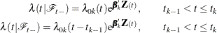
where  is an arbitrary baseline intensity functions, and is a vector of stratum-specific regression coefficients. Here, a subject moves to the kth stratum immediately after his (k – 1) recurrence time and remains there until the kth recurrence occurs or until censorship takes place. For instance, a subject who experiences only one event moves from the
first stratum to the second stratum after the event occurs and remains in the second stratum until the end of the follow-up.
is an arbitrary baseline intensity functions, and is a vector of stratum-specific regression coefficients. Here, a subject moves to the kth stratum immediately after his (k – 1) recurrence time and remains there until the kth recurrence occurs or until censorship takes place. For instance, a subject who experiences only one event moves from the
first stratum to the second stratum after the event occurs and remains in the second stratum until the end of the follow-up.
You can use PROC PHREG to carry out the analyses of the PWP models, but you have to prepare the input data set to provide the correct risk sets. The input data set for analyzing the total time is the same as the AG model with an additional variable to represent the stratum that the subject is in. A subject with K events contributes K + 1 observations to the input data set, one for each stratum that the subject moves to. The input data should contain the following variables:
-
a
TStartvariable to represent the (k – 1) recurrence time or the value 0 if k = 1 -
a
TStopvariable to represent the kth recurrence time or the time of censorship if
-
a
Statusvariable with value 1 if the Time value is a recurrence time and value 0 if the Time value is a censored time -
an
Enumvariable representing the index of the stratum that the subject is in. For a subject who has only one event at and is followed to time
  ,
, Enum=1 for the first observation (whereTime= and Status=1) andEnum=2 for the second observation (whereTime= and Status=0). -
explanatory variables thought to be related to the recurrence times
To analyze gap times, the input data set should also include a GapTime variable that is equal to (TStop – TStart).
Consider the data of two subjects in CGD data described in the previous section:
-
Patients #174054, age 38, in the gamma interferon group had a follow-up time of 293 without any infection.
-
Patient #204001, age 12, in the placebo group had an infection at 219 days, a recurrent infection at 373 days, and a follow-up time of 414 days.
To illustrate, suppose all subjects have at most two observed events. The data for the two subjects in the input data set are as follows:
|
|
|
|
|
|
|
|
|
|---|---|---|---|---|---|---|---|
|
174054 |
0 |
293 |
293 |
0 |
1 |
1 |
38 |
|
204001 |
0 |
219 |
219 |
1 |
1 |
2 |
12 |
|
204001 |
219 |
373 |
154 |
1 |
2 |
2 |
12 |
|
204001 |
373 |
414 |
41 |
0 |
3 |
2 |
12 |
Subject #174054 contributes only one observation to the input data, since there is no observed event. Subject #204001 contributes three observations, since there are two observed events.
To fit the total time model of PWP with stratum-specific slopes, either you can create the stratum-specific explanatory variables
(Trt1, Trt2, and Trt3 for Trt, and Age1, Age2, and Age3 for Age) in a DATA step, or you can specify them in PROC PHREG by using programming statements as follows:
proc phreg;
   model (TStart,TStop)*Status(0)=Trt1 Trt2 Trt3 Age1 Age2 Age3;
   strata Enum;
   Trt1= Trt * (Enum=1);
   Trt2= Trt * (Enum=2);
   Trt3= Trt * (Enum=3);
   Age1= Age * (Enum=1);
   Age2= Age * (Enum=2);
   Age3= Age * (Enum=3);
run;
To fit the total time model of PWP with the common regression coefficients, you specify the following:
proc phreg;
   model (TStart,TStop)*Status(0)=Trt Age;
   strata Enum;
run;
To fit the gap time model of PWP with stratum-specific regression coefficients, you specify the following:
proc phreg;
   model Gaptime*Status(0)=Trt1 Trt2 Trt3 Age1 Age2 Age3;
   strata Enum;
   Trt1= Trt * (Enum=1);
   Trt2= Trt * (Enum=2);
   Trt3= Trt * (Enum=3);
   Age1= Age * (Enum=1);
   Age2= Age * (Enum=2);
   Age3= Age * (Enum=3);
run;
To fit the gap time model of PWP with common regression coefficients, you specify the following:
proc phreg;
   model Gaptime*Status(0)=Trt Age;
   strata Enum;
run;