The PHREG Procedure
- Overview
-
Getting Started

-
SyntaxPROC PHREG StatementASSESS StatementBASELINE StatementBAYES StatementBY StatementCLASS StatementCONTRAST StatementEFFECT StatementESTIMATE StatementFREQ StatementHAZARDRATIO StatementID StatementLSMEANS StatementLSMESTIMATE StatementMODEL StatementOUTPUT StatementProgramming StatementsRANDOM StatementSTRATA StatementSLICE StatementSTORE StatementTEST StatementWEIGHT Statement
-
DetailsFailure Time DistributionTime and CLASS Variables UsagePartial Likelihood Function for the Cox ModelCounting Process Style of InputLeft-Truncation of Failure TimesThe Multiplicative Hazards ModelProportional Rates/Means Models for Recurrent EventsThe Frailty ModelProportional Subdistribution Hazards Model for Competing-Risks DataHazard RatiosNewton-Raphson MethodFirth’s Modification for Maximum Likelihood EstimationRobust Sandwich Variance EstimateTesting the Global Null HypothesisType 3 Tests and Joint TestsConfidence Limits for a Hazard RatioUsing the TEST Statement to Test Linear HypothesesAnalysis of Multivariate Failure Time DataModel Fit StatisticsSchemper-Henderson Predictive MeasureResidualsDiagnostics Based on Weighted ResidualsInfluence of Observations on Overall Fit of the ModelSurvivor Function EstimatorsCaution about Using Survival Data with Left TruncationEffect Selection MethodsAssessment of the Proportional Hazards ModelThe Penalized Partial Likelihood Approach for Fitting Frailty ModelsSpecifics for Bayesian AnalysisComputational ResourcesInput and Output Data SetsDisplayed OutputODS Table NamesODS Graphics
-
ExamplesStepwise RegressionBest Subset SelectionModeling with Categorical PredictorsFirth’s Correction for Monotone LikelihoodConditional Logistic Regression for m:n MatchingModel Using Time-Dependent Explanatory VariablesTime-Dependent Repeated Measurements of a CovariateSurvival CurvesAnalysis of ResidualsAnalysis of Recurrent Events DataAnalysis of Clustered DataModel Assessment Using Cumulative Sums of Martingale ResidualsBayesian Analysis of the Cox ModelBayesian Analysis of Piecewise Exponential ModelAnalysis of Competing-Risks Data
- References
Example 85.12 Model Assessment Using Cumulative Sums of Martingale Residuals
The Mayo liver disease example of Lin, Wei, and Ying (1993) is reproduced here to illustrate the checking of the functional form of a covariate and the assessment of the proportional
hazards assumption. The data represent 418 patients with primary biliary cirrhosis (PBC), among whom 161 had died as of the
date of data listing. A subset of the variables is saved in the SAS data set Liver. The data set contains the following variables:
-
Time, follow-up time, in years -
Status, event indicator with value 1 for death time and value 0 for censored time -
Age, age in years from birth to study registration -
Albumin, serum albumin level, in g/dl -
Bilirubin, serum bilirubin level, in mg/dl -
Edema, edema presence -
Protime, prothrombin time, in seconds
The following statements create the data set Liver:
data Liver;
   input Time Status Age Albumin Bilirubin Edema Protime @@;
   label Time="Follow-up Time in Years";
   Time= Time / 365.25;
   datalines;
  400 1 58.7652 2.60 14.5 1.0 12.2 4500 0 56.4463 4.14  1.1 0.0 10.6
 1012 1 70.0726 3.48  1.4 0.5 12.0 1925 1 54.7406 2.54  1.8 0.5 10.3
 1504 0 38.1054 3.53  3.4 0.0 10.9 2503 1 66.2587 3.98  0.8 0.0 11.0
 1832 0 55.5346 4.09  1.0 0.0  9.7 2466 1 53.0568 4.00  0.3 0.0 11.0
 2400 1 42.5079 3.08  3.2 0.0 11.0   51 1 70.5599 2.74 12.6 1.0 11.5
 3762 1 53.7139 4.16  1.4 0.0 12.0  304 1 59.1376 3.52  3.6 0.0 13.6
 3577 0 45.6893 3.85  0.7 0.0 10.6 1217 1 56.2218 2.27  0.8 1.0 11.0
 3584 1 64.6461 3.87  0.8 0.0 11.0 3672 0 40.4435 3.66  0.7 0.0 10.8

   ... more lines ...

  989 0 35.0000 3.23  0.7 0.0 10.8  681 1 67.0000 2.96  1.2 0.0 10.9
 1103 0 39.0000 3.83  0.9 0.0 11.2 1055 0 57.0000 3.42  1.6 0.0  9.9
  691 0 58.0000 3.75  0.8 0.0 10.4  976 0 53.0000 3.29  0.7 0.0 10.6
;
Consider fitting a Cox model for the survival time of the PCB patients with the covariates Bilirubin, log(Protime), log(Albumin), Age, and Edema. The log transform, which is often applied to blood chemistry measurements, is deliberately not employed for Bilirubin. It is of interest to assess the functional form of the variable Bilirubin in the Cox model. The specifications are as follows:
ods graphics on;
proc phreg data=Liver;
   model Time*Status(0)=Bilirubin logProtime logAlbumin Age Edema;
   logProtime=log(Protime);
   logAlbumin=log(Albumin);
   assess var=(Bilirubin) /  resample seed=7548;
run;
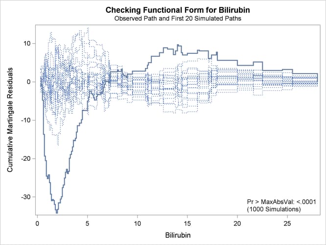
The ASSESS statement creates a plot of the cumulative martingale residuals against the values of the covariate Bilirubin, which is specified in the VAR= option. The RESAMPLE option computes the p-value of a Kolmogorov-type supremum test based on a sample of 1,000 simulated residual patterns.
Parameter estimates of the model fit are shown in Output 85.12.1. The plot in Output 85.12.2 displays the observed cumulative martingale residual process for Bilirubin together with 20 simulated realizations from the null distribution. When ODS Graphics is enabled, this graphical display
is requested by specifying the ASSESS statement. It is obvious that the observed process is atypical compared to the simulated
realizations. Also, none of the 1,000 simulated realizations has an absolute maximum exceeding that of the observed cumulative
martingale residual process. Both the graphical and numerical results indicate that a transform is deemed necessary for Bilirubin in the model.
Output 85.12.1: Cox Model with Bilirubin as a Covariate
| Analysis of Maximum Likelihood Estimates | ||||||
|---|---|---|---|---|---|---|
| Parameter | DF | Parameter Estimate |
Standard Error |
Chi-Square | Pr > ChiSq | Hazard Ratio |
| Bilirubin | 1 | 0.11733 | 0.01298 | 81.7567 | <.0001 | 1.124 |
| logProtime | 1 | 2.77581 | 0.71482 | 15.0794 | 0.0001 | 16.052 |
| logAlbumin | 1 | -3.17195 | 0.62945 | 25.3939 | <.0001 | 0.042 |
| Age | 1 | 0.03779 | 0.00805 | 22.0288 | <.0001 | 1.039 |
| Edema | 1 | 0.84772 | 0.28125 | 9.0850 | 0.0026 | 2.334 |
Output 85.12.2: Cumulative Martingale Residuals vs Bilirubin
The cumulative martingale residual plots in Output 85.12.3 provide guidance in suggesting a more appropriate functional form for a covariate. The four curves were created from simple forms of misspecification by using 10,000 simulated times from a exponential model with 20% censoring. The true and fitted models are shown in Table 85.19. The following statements produce Output 85.12.3.
data sim(drop=tmp);
   p = 1 / 91;
   seed = 1;
   do n = 1 to 10000;
      x1 = rantbl( seed, p, p, p, p, p, p, p, p, p, p,
                            p, p, p, p, p, p, p, p, p, p,
                            p, p, p, p, p, p, p, p, p, p,
                            p, p, p, p, p, p, p, p, p, p,
                            p, p, p, p, p, p, p, p, p, p,
                            p, p, p, p, p, p, p, p, p, p,
                            p, p, p, p, p, p, p, p, p, p,
                            p, p, p, p, p, p, p, p, p, p,
                            p, p, p, p, p, p, p, p, p, p );

      x1 = 1 + ( x1 - 1 ) / 10;
      x2= x1 * x1;
      x3= x1 * x2;
      status= rantbl(seed, .8);
      tmp= log(1-ranuni(seed));
      t1= -exp(-log(x1)) * tmp;
      t2= -exp(-.1*(x1+x2)) * tmp;
      t3= -exp(-.01*(x1+x2+x3)) * tmp;
      tt= -exp(-(x1>5)) * tmp;
      output;
   end;
run;


proc sort data=sim;
   by x1;
run;

proc phreg data=sim noprint;
   model t1*status(2)=x1;
   output out=out1 resmart=resmart;
run;

proc phreg data=sim noprint;
   model t2*status(2)=x1;
   output out=out2 resmart=resmart;
run;


proc phreg data=sim noprint;
   model t3*status(2)=x1 x2;
   output out=out3 resmart=resmart;
run;

proc phreg data=sim noprint;
   model tt*status(2)=x1;
   output out=out4 resmart=resmart;
run;

data out1(keep=x1 cresid1);
   retain cresid1 0;
   set out1;
   by x1;
   cresid1 + resmart;
   if last.x1  then output;
run;

data out2(keep=x1 cresid2);
   retain cresid2 0;
   set out2;
   by x1;
   cresid2 + resmart;
   if last.x1  then output;
run;


data out3(keep=x1 cresid3);
   retain cresid3 0;
   set out3;
   by x1;
   cresid3 + resmart;
   if last.x1  then output;
run;

data out4(keep=x1 cresid4);
   retain cresid4 0;
   set out4;
   by x1;
   cresid4 + resmart;
   if last.x1  then output;
run;

data all;
   set out1;
   set out2;
   set out3;
   set out4;
run;

proc template;
   define statgraph MisSpecification;
      BeginGraph;
         entrytitle "Covariate Misspecification";
         layout lattice / columns=2 rows=2 columndatarange=unionall;

            columnaxes;
               columnaxis / display=(ticks tickvalues label) label="x";
               columnaxis / display=(ticks tickvalues label) label="x";
            endcolumnaxes;

            cell;
               cellheader;
                  entry "(a) Data: log(X), Model: X";
               endcellheader;
               layout overlay / xaxisopts=(display=none)
                                yaxisopts=(label="Cumulative Residual");
                  seriesplot y=cresid1 x=x1 / lineattrs=GraphFit;
               endlayout;
            endcell;

            cell;
               cellheader;
                  entry "(b) Data: X*X, Model: X";
               endcellheader;
               layout overlay / xaxisopts=(display=none)
                                yaxisopts=(label=" ");
                  seriesplot y=cresid2 x=x1 / lineattrs=GraphFit;
               endlayout;
            endcell;

            cell;
               cellheader;
                  entry "(c) Data: X*X*X, Model: X*X";
               endcellheader;
               layout overlay / xaxisopts=(display=none)
                                yaxisopts=(label="Cumulative Residual");
                  seriesplot y=cresid3 x=x1 / lineattrs=GraphFit;
               endlayout;
            endcell;

            cell;
               cellheader;
                  entry "(d) Data: I(X>5), Model: X";
               endcellheader;
               layout overlay / xaxisopts=(display=none)
                                yaxisopts=(label=" ");
                  seriesplot y=cresid4 x=x1 / lineattrs=GraphFit;
               endlayout;
            endcell;

         endlayout;
      EndGraph;
   end;
run;

proc sgrender data=all template=MisSpecification;
run;
Output 85.12.3: Typical Cumulative Residual Plot Patterns
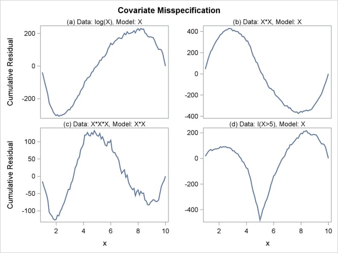
Table 85.19: Model Misspecifications
|
Plot |
Data |
Fitted Model |
|---|---|---|
|
(a) |
log(X) |
X |
|
(b) |
|
X |
|
(c) |
|
|
|
(d) |
|
X |


The curve of observed cumulative martingale residuals in Output 85.12.2 most resembles the behavior of the curve in plot (a) of Output 85.12.3, indicating that log(Bilirubin) might be a more appropriate term in the model than Bilirubin.
Next, the analysis of the natural history of the PBC is repeated with log(Bilirubin) replacing Bilirubin, and the functional form of log(Bilirubin) is assessed. Also assessed is the proportional hazards assumption for the Cox model. The analysis is carried out by the
following statements:
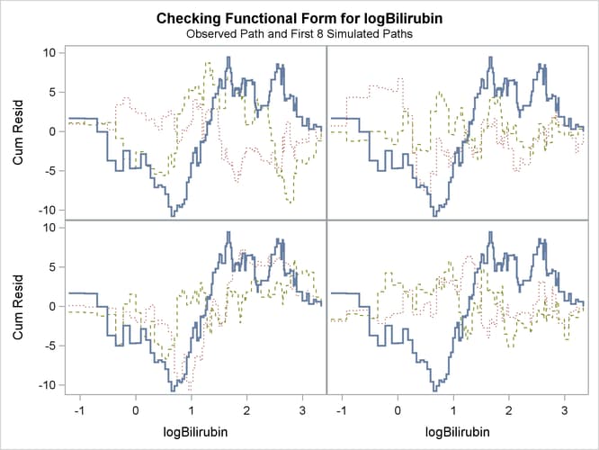
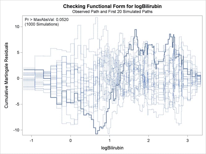
proc phreg data=Liver;
   model Time*Status(0)=logBilirubin logProtime logAlbumin Age Edema;
   logBilirubin=log(Bilirubin);
   logProtime=log(Protime);
   logAlbumin=log(Albumin);
   assess var=(logBilirubin) ph / crpanel resample seed=19;
run;
The SEED= option specifies a integer seed for generating random numbers. The CRPANEL option in the ASSESS statement requests a panel of four plots. Each plot displays the observed cumulative martingale residual process along with two simulated realizations. The PH option checks the proportional hazards assumption of the model by plotting the observed standardized score process with 20 simulated realizations for each covariate in the model.
Output 85.12.4 displays the parameter estimates of the fitted model. The cumulative martingale residual plots in Output 85.12.5 and Output 85.12.6 show that the observed martingale residual process is more typical of the simulated realizations. The p-value for the Kolmogorov-type supremum test based on 1,000 simulations is 0.052, indicating that the log transform is a much
improved functional form for Bilirubin.
Output 85.12.4: Model with log(Bilirubin) as a Covariate
| Analysis of Maximum Likelihood Estimates | ||||||
|---|---|---|---|---|---|---|
| Parameter | DF | Parameter Estimate |
Standard Error |
Chi-Square | Pr > ChiSq | Hazard Ratio |
| logBilirubin | 1 | 0.87072 | 0.08263 | 111.0484 | <.0001 | 2.389 |
| logProtime | 1 | 2.37789 | 0.76674 | 9.6181 | 0.0019 | 10.782 |
| logAlbumin | 1 | -2.53264 | 0.64819 | 15.2664 | <.0001 | 0.079 |
| Age | 1 | 0.03940 | 0.00765 | 26.5306 | <.0001 | 1.040 |
| Edema | 1 | 0.85934 | 0.27114 | 10.0447 | 0.0015 | 2.362 |
Output 85.12.5: Panel Plot of Cumulative Martingale Residuals versus log(Bilirubin)
Output 85.12.6: Cumulative Martingale Residuals versus log(Bilirubin)
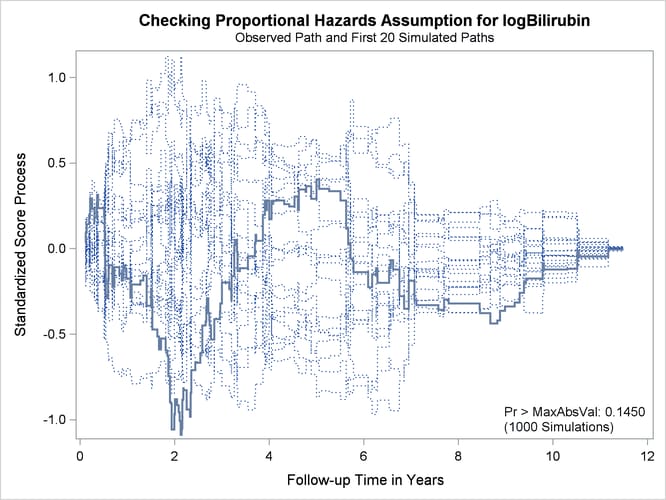
Output 85.12.7 and Output 85.12.8 display the results of proportional hazards assumption assessment for log(Bilirubin) and log(Protime), respectively. The latter plot reveals nonproportional hazards for log(Protime).
Output 85.12.7: Standardized Score Process for log(Bilirubin)
[
Output 85.12.8: Standardized Score Process for log(Protime)
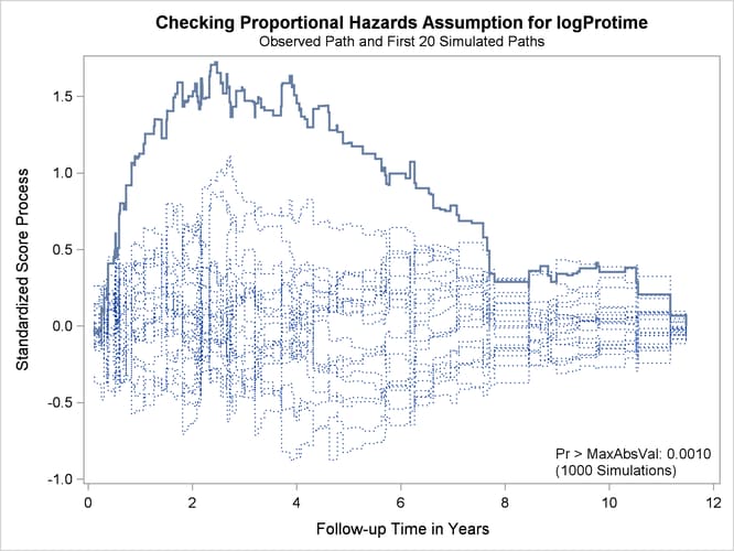
Plots for log(Albumin), Age, and Edema are not shown here. The Kolmogorov-type supremum test results for all the covariates are shown in Output 85.12.9. In addition to log(Protime), the proportional hazards assumption appears to be violated for Edema.
Output 85.12.9: Kolmogorov-Type Supremum Tests for Proportional Hazards Assumption