The PHREG Procedure
- Overview
-
Getting Started

-
SyntaxPROC PHREG StatementASSESS StatementBASELINE StatementBAYES StatementBY StatementCLASS StatementCONTRAST StatementEFFECT StatementESTIMATE StatementFREQ StatementHAZARDRATIO StatementID StatementLSMEANS StatementLSMESTIMATE StatementMODEL StatementOUTPUT StatementProgramming StatementsRANDOM StatementSTRATA StatementSLICE StatementSTORE StatementTEST StatementWEIGHT Statement
-
DetailsFailure Time DistributionTime and CLASS Variables UsagePartial Likelihood Function for the Cox ModelCounting Process Style of InputLeft-Truncation of Failure TimesThe Multiplicative Hazards ModelProportional Rates/Means Models for Recurrent EventsThe Frailty ModelProportional Subdistribution Hazards Model for Competing-Risks DataHazard RatiosNewton-Raphson MethodFirth’s Modification for Maximum Likelihood EstimationRobust Sandwich Variance EstimateTesting the Global Null HypothesisType 3 Tests and Joint TestsConfidence Limits for a Hazard RatioUsing the TEST Statement to Test Linear HypothesesAnalysis of Multivariate Failure Time DataModel Fit StatisticsSchemper-Henderson Predictive MeasureResidualsDiagnostics Based on Weighted ResidualsInfluence of Observations on Overall Fit of the ModelSurvivor Function EstimatorsCaution about Using Survival Data with Left TruncationEffect Selection MethodsAssessment of the Proportional Hazards ModelThe Penalized Partial Likelihood Approach for Fitting Frailty ModelsSpecifics for Bayesian AnalysisComputational ResourcesInput and Output Data SetsDisplayed OutputODS Table NamesODS Graphics
-
ExamplesStepwise RegressionBest Subset SelectionModeling with Categorical PredictorsFirth’s Correction for Monotone LikelihoodConditional Logistic Regression for m:n MatchingModel Using Time-Dependent Explanatory VariablesTime-Dependent Repeated Measurements of a CovariateSurvival CurvesAnalysis of ResidualsAnalysis of Recurrent Events DataAnalysis of Clustered DataModel Assessment Using Cumulative Sums of Martingale ResidualsBayesian Analysis of the Cox ModelBayesian Analysis of Piecewise Exponential ModelAnalysis of Competing-Risks Data
- References
The Penalized Partial Likelihood Approach for Fitting Frailty Models
Let  be the vector of random components for the s clusters.
Gamma Frailty Model
Assume each  has an independent and identically distributed gamma distribution with mean 1 and a common unknown variance
  ; that is, is iid
  . The penalty function is
![\[ - \frac{1}{\theta } \sum _{i=1}^ s \biggl ( \gamma _ i - \mr{e}^{\gamma _ i} \biggr ) \]](images/statug_phreg0746.png)
plus a function of . The penalized partial log likelihood is given by
![\[ l_{p}(\bbeta , \bgamma ,\theta ) =l_{\mr{partial}}(\bbeta , \bgamma ) + \frac{1}{\theta } \sum _{i=1}^ s \biggl ( \gamma _ i - \mr{e}^{\gamma _ i} \biggr ) \]](images/statug_phreg0747.png)
where  is the log of any of the partial likelihoods in the sections Partial Likelihood Function for the Cox Model and The Multiplicative Hazards Model.
The profile marginal log-likelihood of this shared frailty model (Therneau and Grambsch 2000, pp. 257–258) is
![\[ l_ m(\theta ) = l_{p}(\hat{\bbeta }(\theta ), \hat{\bgamma }(\theta ),\theta ) + \sum _{i=1}^ s \left\{ \theta ^{-1} - ( \theta ^{-1} + d_ i)\log \left[ \theta ^{-1} + d_ i \right] + \theta ^{-1}\log (\theta ^{-1}) + \log \left[ \frac{\Gamma (\theta ^{-1}+d_ i)}{\Gamma (\theta ^{-1})}\right] \right\} \]](images/statug_phreg0749.png)
where  is the number of events in the ith cluster.
The maximization of this approximate likelihood is a doubly iterative process that alternates between the following two steps:
-
For a provisional value of
, the best linear unbiased predictors (BLUP) of  and
and  are computed by maximizing the penalized partial log-likelihood
  . The marginal likelihood is evaluated. This constitutes the inner loop.
-
A new value of
is obtained by the golden section search based on the marginal likelihood of all the previous iterations. This constitutes
the outer loop.
The outer loop is iterated until the bracketing interval of is small.
Lognormal Frailty Model
With each  having a zero-mean normal distribution and a common variance , the penalty function is
![\[ \frac{1}{2\theta }\bgamma ’\bgamma \]](images/statug_phreg0752.png)
plus a function of . The penalized partial log likelihood is given by
![\[ l_{p}(\bbeta , \bgamma ,\theta ) =l_{\mr{partial}}(\bbeta , \bgamma ) - \frac{1}{2\theta }\bgamma ’\bgamma \]](images/statug_phreg0753.png)
where  is the log of any of the partial likelihoods in the sections Partial Likelihood Function for the Cox Model and The Multiplicative Hazards Model.
For a given , let  be the negative Hessian of the penalized partial log likelihood ; that is,
![\[ \bH = \bH (\bbeta ,\bgamma )=\left[ \begin{array}{cc} \mc{\bH }_{11} & \mc{\bH }_{12} \\ \bH _{21} & \bH _{22} \\ \end{array} \right] \]](images/statug_phreg0755.png)
where 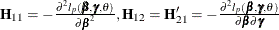 , and
, and 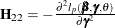 .
.
The marginal log likelihood of this shared frailty model is
![\[ l_ m(\bbeta ,\theta ) = -\frac{1}{2} \log (\theta ^ s) + \log \biggr [\int \mr{e}^{l_ p(\bbeta ,\bgamma ,\theta )}d\bgamma \biggr ] \]](images/statug_phreg0758.png)
Using a Laplace approximation to the integral as in Breslow and Clayton (1993), an approximate marginal log likelihood (Ripatti and Palmgren 2000; Therneau and Grambsch 2000) is given by
![\[ l_ m(\bbeta ,\theta ) \approx -\frac{1}{2} \log (\theta ^ s) -\frac{1}{2} \log (|\bH _{22}(\bbeta ,\tilde{\bgamma },\theta )|) -l_ p(\bbeta ,\tilde{\bgamma },\theta ) \]](images/statug_phreg0759.png)
The maximization of this approximate likelihood is a doubly iterative process that alternates between the following two steps:
-
For a provisional value of
, PROC PHREG computes the best linear unbiased predictors (BLUP) of and by maximizing the penalized partial log likelihood . This constitutes the inner loop.
-
For
and fixed at the BLUP values, PROC PHREG estimates by maximizing the approximate marginal likelihood  . This constitutes the outer loop.
The outer loop is iterated until the difference between two successive estimates of is small.
The ML estimate of is
![\[ \hat{\theta }= \frac{\hat{\bgamma }'\hat{\bgamma } + \mr{trace}(\bH _{22}^{-1})}{s} \]](images/statug_phreg0761.png)
The variance for  is
is
![\[ \mr{var}(\hat{\theta }) = 2 \hat{\theta } \biggl [s + \frac{1}{\hat{\theta }^2}\mr{trace}(\bH _{22}^{-1}\bH _{22}^{-1}) -\frac{2}{\hat{\theta }}\mr{trace}(\bH _{22}^{-1}) \biggr ]^{-1} \]](images/statug_phreg0763.png)
The REML estimation of is obtained by replacing  by
by  .
.
The inverse of the final matrix is used as the variance estimate of  .
.
The final BLUP estimates of the random components  can be displayed by using the SOLUTION option in the RANDOM statement. Also displayed are estimates of the lognormal frailties,
which are the exponentiated estimates of the BLUP estimates.
can be displayed by using the SOLUTION option in the RANDOM statement. Also displayed are estimates of the lognormal frailties,
which are the exponentiated estimates of the BLUP estimates.
Wald-Type Tests for Penalized Models
Let  be the negative Hessian of the partial log likelihood
  :
:
![\[ \bI = \left[ \begin{array}{cc} \bI _{11} & \bI _{12} \\ \bI _{21} & \bI _{22} \\ \end{array} \right] \]](images/statug_phreg0768.png)
where 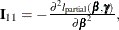
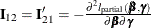 , and
, and 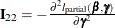 . Write
  . The Wald-type chi-square statistic for testing
  is
is
![\[ (\bC \hat{\btau })’ (\bC \bH ^{-1} \bC ’)^{-1} (\bC \hat{\btau }) \]](images/statug_phreg0774.png)
Let be the negative Hessian of the penalized partial log likelihood at the ML estimate ; that is, 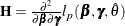 . Let
. Let  . Gray (1992) recommends the following generalized degrees of freedom for the Wald test:
![\[ \mr{DF}=\mr{trace}[(\bC \bH ^{-1}\bC ’)^{-1}\bC \bV \bC ’)] \]](images/statug_phreg0777.png)
See Therneau and Grambsch (2000, Section 5.8) for a discussion of this Wald-type test.
PROC PHREG uses the label "Adjusted DF" to represent this generalized degrees of freedom in the output.