The CALIS Procedure
-
Overview

-
Getting Started
-
SyntaxClasses of Statements in PROC CALISSingle-Group Analysis SyntaxMultiple-Group Multiple-Model Analysis SyntaxPROC CALIS StatementBOUNDS StatementBY StatementCOSAN StatementCOV StatementDETERM StatementEFFPART StatementFACTOR StatementFITINDEX StatementFREQ StatementGROUP StatementLINCON StatementLINEQS StatementLISMOD StatementLMTESTS StatementMATRIX StatementMEAN StatementMODEL StatementMSTRUCT StatementNLINCON StatementNLOPTIONS StatementOUTFILES StatementPARAMETERS StatementPARTIAL StatementPATH StatementPATHDIAGRAM StatementPCOV StatementPVAR StatementRAM StatementREFMODEL StatementRENAMEPARM StatementSAS Programming StatementsSIMTESTS StatementSTD StatementSTRUCTEQ StatementTESTFUNC StatementVAR StatementVARIANCE StatementVARNAMES StatementWEIGHT Statement
-
DetailsInput Data SetsOutput Data SetsDefault Analysis Type and Default ParameterizationThe COSAN ModelThe FACTOR ModelThe LINEQS ModelThe LISMOD Model and SubmodelsThe MSTRUCT ModelThe PATH ModelThe RAM ModelNaming Variables and ParametersSetting Constraints on ParametersAutomatic Variable SelectionPath Diagrams: Layout Algorithms, Default Settings, and CustomizationEstimation CriteriaRelationships among Estimation CriteriaGradient, Hessian, Information Matrix, and Approximate Standard ErrorsCounting the Degrees of FreedomAssessment of FitCase-Level Residuals, Outliers, Leverage Observations, and Residual DiagnosticsLatent Variable ScoresTotal, Direct, and Indirect EffectsStandardized SolutionsModification IndicesMissing Values and the Analysis of Missing PatternsMeasures of Multivariate KurtosisInitial EstimatesUse of Optimization TechniquesComputational ProblemsDisplayed OutputODS Table NamesODS Graphics
-
ExamplesEstimating Covariances and CorrelationsEstimating Covariances and Means SimultaneouslyTesting Uncorrelatedness of VariablesTesting Covariance PatternsTesting Some Standard Covariance Pattern HypothesesLinear Regression ModelMultivariate Regression ModelsMeasurement Error ModelsTesting Specific Measurement Error ModelsMeasurement Error Models with Multiple PredictorsMeasurement Error Models Specified As Linear EquationsConfirmatory Factor ModelsConfirmatory Factor Models: Some VariationsResidual Diagnostics and Robust EstimationThe Full Information Maximum Likelihood MethodComparing the ML and FIML EstimationPath Analysis: Stability of AlienationSimultaneous Equations with Mean Structures and Reciprocal PathsFitting Direct Covariance StructuresConfirmatory Factor Analysis: Cognitive AbilitiesTesting Equality of Two Covariance Matrices Using a Multiple-Group AnalysisTesting Equality of Covariance and Mean Matrices between Independent GroupsIllustrating Various General Modeling LanguagesTesting Competing Path Models for the Career Aspiration DataFitting a Latent Growth Curve ModelHigher-Order and Hierarchical Factor ModelsLinear Relations among Factor LoadingsMultiple-Group Model for Purchasing BehaviorFitting the RAM and EQS Models by the COSAN Modeling LanguageSecond-Order Confirmatory Factor AnalysisLinear Relations among Factor Loadings: COSAN Model SpecificationOrdinal Relations among Factor LoadingsLongitudinal Factor Analysis
- References
Example 29.28 Multiple-Group Model for Purchasing Behavior
In this example, data were collected from customers who made purchases from a retail company during years 2002 and 2003. A two-group structural equation model is fitted to the data.
The variables are:
- Spend02:
-
total purchase amount in 2002
- Spend03:
-
total purchase amount in 2003
- Courtesy:
-
rating of the courtesy of the customer service
- Responsive:
-
rating of the responsiveness of the customer service
- Helpful:
-
rating of the helpfulness of the customer service
- Delivery:
-
rating of the timeliness of the delivery
- Pricing:
-
rating of the product pricing
- Availability:
-
rating of the product availability
- Quality:
-
rating of the product quality
For the ratings scales, nine-point scales were used. Customers could respond 1 to 9 on these scales, with 1 representing "extremely
unsatisfied" and 9 representing "extremely satisfied." Data were collected from two different regions, which are labeled as
Region 1 ( ) and Region 2 (
 ), respectively. The ratings were collected at the end of year 2002 so that they represent customers’ purchasing experience
in year 2002.
), respectively. The ratings were collected at the end of year 2002 so that they represent customers’ purchasing experience
in year 2002.
The central questions of the study are:
-
How does the overall customer service affect the current purchases and predict future purchases?
-
How does the overall product quality affect the current purchases and predict future purchases?
-
Do current purchases predict future purchases?
-
Do the two regions have different structural models for predicting the purchases?
In stating these research questions, you use several constructs that might or might not correspond to objective measurements.
Current and future purchases are certainly measurable directly by the spending of the customers. That is, because customer
service and product satisfaction and quality were surveyed between 2002 and 2003, Spend02 represents current purchases and Spend03 represents future purchases in the study. Both variables Spend02 and Spend03 are objective measurements without measurement errors. All you need to do is to extract the information from the transaction
records. But how about hypothetical constructs such as customer service quality and product quality? How would you measure
them in the model?
In measuring these hypothetical constructs, you might ask customers’ perception about the service or product quality directly in a single question. A simple survey with two questions about the customer service and product qualities could then be what you need. These questions are called indicators (or indicator variables) of the underlying constructs. However, using just one indicator (question) for each of these hypothetical constructs would be quite unreliable—that is, measurement errors might dominate in the data collection process. Therefore, multiple indicators are usually recommended for measuring such hypothetical constructs.
There are two main advantages of using multiple indicators for hypothetical constructs. The first one is conceptual and the other is statistical and mathematical.
First, hypothetical constructs might conceptually be multifaceted themselves. Measuring a hypothetical construct by a single indicator does not capture the full meaning of the construct. For example, the product quality might refer to the durability of the product, the outlook of the product, the pricing of the product, and the availability of product, among others. The customer service quality might refer to the politeness of the customer service, the timeliness of the delivery, and the responsiveness of customer services, among others. Therefore, multiple indicators for a single hypothetical construct might be necessary if you want to cover the multifaceted aspects of a given hypothetical construct.
Second, from a statistical point of view, the reliability would be higher if you combine correlated indicators for a construct than if you use a single indicator only. Therefore, combining correlated indicators would lead to more accurate and reliable results.
One way to combine correlated indicators is to use a simple sum of them to represent the underlying hypothetical construct. However, a better way is to use the structural equation modeling technique that represents each indicator (variable) as a function of the underlying hypothetical construct plus an error term. In structural equation modeling, hypothetical constructs are constructed as latent factors, which are unobserved systematic (that is, non-error) variables. Theoretically, latent factors are free from measurement errors, and so the estimation through the structural equation modeling technique is more accurate than if you just use simple sums of indicators to represent hypothetical constructs. Therefore, a structural equation modeling approach is the method of the choice in the current analysis.
In practice, you must also make sure that there are enough indicators for the identification of the underlying latent factor, and hence the identification of the entire model. Necessary and sufficient rules for identification are very complicated to describe and are out of the scope of the current discussion (however, see Bollen 1989b for discussions of identification rules for various classes of structural equation models). Some simple rules of thumb might be useful as a guidance. For example, for unconstrained situations, you should at least have three indicators (variables) measured for a latent factor. Unfortunately, these rules of thumb do not guarantee identification in every case.
In this example, Service and Product are latent factors in the structural equation model which represent service and product qualities, respectively. In the model,
these two latent factors are reflected by the ratings of the customers. Ratings on the Courtesy, Responsive, Helpful, and Delivery scales are indicators of Service. Ratings on the Pricing, Availability, and Quality scales are indicators of Product (that is, product quality).
A Path Diagram
A path diagram shown in Output 29.28.1 represents the structural equation model for the purchase behavior. Observed or manifest variables are represented by rectangles,
and latent variables are represented by ovals. As mentioned, two latent variables (factors), Service and Product, are created as overall measures of customer service and product qualities, respectively.
Output 29.28.1: Path Diagram of Purchasing Behavior
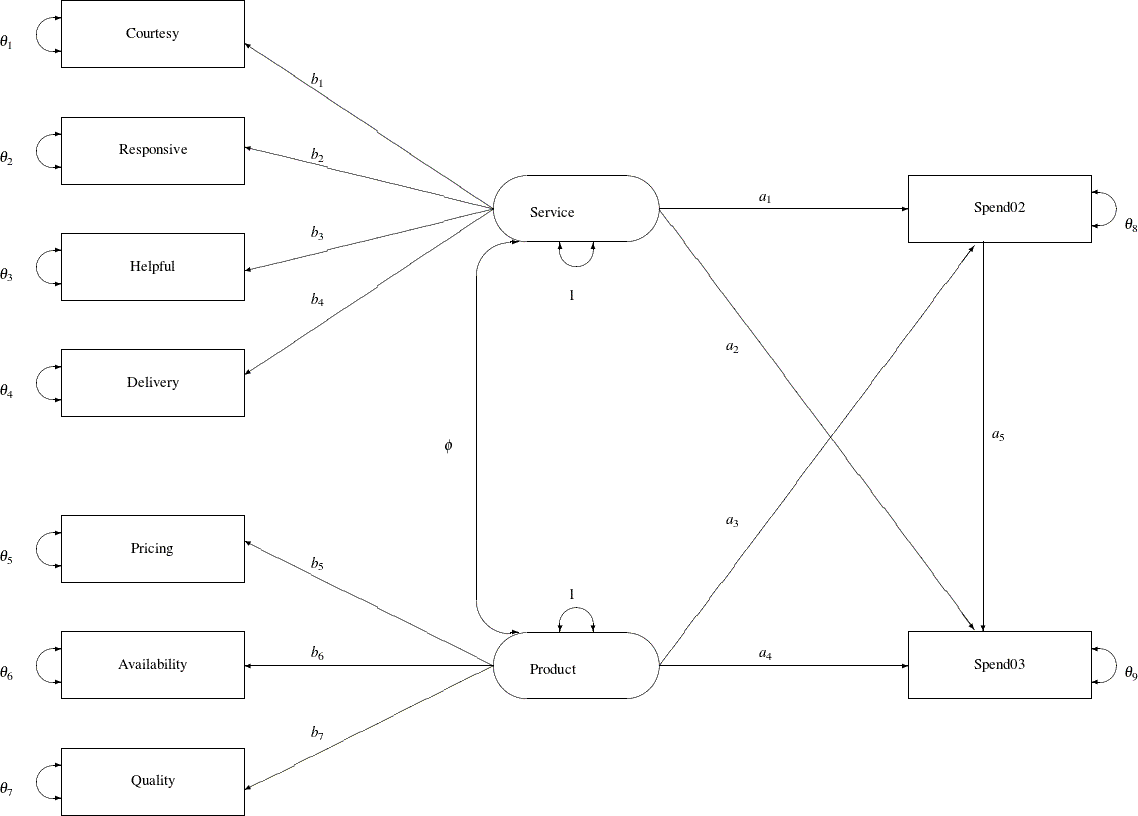
The left part of the diagram represents the measurement model of the latent variables. The Service factor has four indicators: Courtesy, Responsive, Helpful, and Delivery. The path coefficients to these observed variables from the Service factor are  ,
,  ,
,  , and
, and  , respectively. Similarly, the
 Product variable has three indicators: Pricing, Availability, and Quality, with path coefficients  ,
,  , and
, and  , respectively.
The two latent factors are predictors of the purchase amounts Spend02 and Spend03. In addition, Spend02 also serves as a predictor of Spend03. Path coefficients (effects) for this part of functional relationships are represented by a1–a5 in the diagram.
Each variable in the path diagram has a variance parameter. For endogenous or dependent variables, which serve as outcome
variables in the model, the variance parameters are the error variances that are not accounted for by the predictors. For
example, in the current model all observed variables are endogenous variables. The double-headed arrows that are attached
to these variables represent error variances. In the diagram,  to
to  are the names of these error variance parameters. For exogenous or independent variables, which never serve as outcome variables
in the model, the variance parameters are the (total) variances of these variables. For example, in the diagram the double-headed
arrows that are attached to
are the names of these error variance parameters. For exogenous or independent variables, which never serve as outcome variables
in the model, the variance parameters are the (total) variances of these variables. For example, in the diagram the double-headed
arrows that are attached to Service and Product represent the variances of these two latent variables. In the current model, both of these variances are fixed at one.
When the double-headed arrows point to two variables, they represent covariances in the path diagram. For example, in Output 29.28.1 the covariance between Service and Product is represented by the parameter  .
.
The Basic Path Model Specification
For the moment, it is hypothesized that both 'Region 1' and 'Region 2' data are fitted by the same model as shown in Output 29.28.1. Once the path diagram is drawn, it is readily translated into the PATH modeling language. See the PATH statement for details about how to use the PATH modeling language to specify structural equation models.
To represent all the features in the path diagram in the PATH model language, you can use the following specification:
path
   Service ===> Spend02      = a1,
   Service ===> Spend03      = a1,
   Product ===> Spend02      = a3,
   Product ===> Spend03      = a4,
   Spend02 ===> Spend03      = a5,
   Service ===> Courtesy     = b1,
   Service ===> Responsive   = b2,
   Service ===> Helpful      = b3,
   Service ===> Delivery     = b4,
   Product ===> Pricing      = b5,
   Product ===> Availability = b6,
   Product ===> Quality      = b7;
pvar
   Courtesy Responsive Helpful
   Delivery Pricing
   Availability Quality = theta01-theta07,
   Spend02 = theta08,
   Spend03 = theta09,
   Service Product = 2 * 1.;
pcov
   Service Product = phi;
The PATH
statement captures all the path coefficient specifications and the direction of the paths (single-headed arrows) in the path
diagram. The first five paths define how Spend02 and Spend03 are predicted from the latent variables Service, Product, and Spend02. The next seven paths define the measurement model, which shows how the latent variables in the model relate to the observed
indicator variables.
The PVAR
statement captures the specification of the error variances and the variances of exogenous variables (that is, the double-headed
arrows in the path diagram). The PCOV
statement captures the specification of covariance between the two latent variables in the model (which is represented by
the double-headed arrow that connects Service and Product in the path diagram).
You can also use the following simpler version of the PATH model specification for the path diagram:
path
   Service ===> Spend02  Spend03      ,
   Product ===> Spend02  Spend03      ,
   Spend02 ===> Spend03               ,
   Service ===> Courtesy Responsive
                Helpful Delivery      ,
   Product ===> Pricing  Availability
                Quality               ;
pvar
   Courtesy Responsive Helpful Delivery Pricing
   Availability Quality Spend02 Spend03,
   Service Product = 2 * 1.;
pcov
   Service Product;
There are two simplifications in this PATH model specification. First, you do not need to specify the parameter names if they
are unconstrained in the model. For example, parameter a1 in the model is unique to the path effect from Service to Spend02. You do not need to name this effect because it is not constrained to be the same as any other parameter in the model. Similar,
all the path coefficients (effects), error variances, and covariances in the path diagram are not constrained. Therefore,
you can omit all the corresponding parameter name specifications in the PATH model specification. The only exceptions are
the variances of Service and Product. Both are fixed constants 1 in the path diagram, and so you must specify them explicitly in the PVAR statement.
Second, you use a condensed way to specify the paths. In the first three path entries of the PATH statement, you specify how
Spend02 and Spend03 are predicted from the latent variables Service, Product, and Spend02. Notice that in each path entry, you can define more than one path (single-headed arrow relationship). For example, in the
first path entry, you specify two paths: one is Service===>Spend02 and the other is Service===>Spend03. In the last two path entries of the PATH statement, you define the relationships between the two latent constructs Spend and Service and their measured indicators. Each of these path entries specifies multiple paths (single-headed arrow relationships).
You use this simplified PATH specifications in the subsequent analysis.
A Restrictive Model with Invariant Mean and Covariance Structures
In this section, you fit a mean and covariance structure model to the data from two regions, as shows in the following DATA steps:
data region1(type=cov);
   input _type_ $6. _name_ $12. Spend02 Spend03 Courtesy Responsive
         Helpful Delivery Pricing Availability Quality;
   datalines;
COV   Spend02      14.428  2.206  0.439 0.520 0.459 0.498 0.635 0.642 0.769
COV   Spend03       2.206 14.178  0.540 0.665 0.560 0.622 0.535 0.588 0.715
COV   Courtesy      0.439  0.540  1.642 0.541 0.473 0.506 0.109 0.120 0.126
COV   Responsive    0.520  0.665  0.541 2.977 0.582 0.629 0.119 0.253 0.184
COV   Helpful       0.459  0.560  0.473 0.582 2.801 0.546 0.113 0.121 0.139
COV   Delivery      0.498  0.622  0.506 0.629 0.546 3.830 0.120 0.132 0.145
COV   Pricing       0.635  0.535  0.109 0.119 0.113 0.120 2.152 0.491 0.538
COV   Availability  0.642  0.588  0.120 0.253 0.121 0.132 0.491 2.372 0.589
COV   Quality       0.769  0.715  0.126 0.184 0.139 0.145 0.538 0.589 2.753
MEAN     .        183.500 301.921 4.312 4.724 3.921 4.357 6.144 4.994 5.971
;

data region2(type=cov);
   input _type_ $6. _name_ $12. Spend02 Spend03 Courtesy Responsive
         Helpful Delivery Pricing Availability Quality;
   datalines;
COV   Spend02       14.489   2.193 0.442 0.541 0.469 0.508 0.637 0.675 0.769
COV   Spend03        2.193  14.168 0.542 0.663 0.574 0.623 0.607 0.642 0.732
COV   Courtesy       0.442   0.542 3.282 0.883 0.477 0.120 0.248 0.283 0.387
COV   Responsive     0.541   0.663 0.883 2.717 0.477 0.601 0.421 0.104 0.105
COV   Helpful        0.469   0.574 0.477 0.477 2.018 0.507 0.187 0.162 0.205
COV   Delivery       0.508   0.623 0.120 0.601 0.507 2.999 0.179 0.334 0.099
COV   Pricing        0.637   0.607 0.248 0.421 0.187 0.179 2.512 0.477 0.423
COV   Availability   0.675   0.642 0.283 0.104 0.162 0.334 0.477 2.085 0.675
COV   Quality        0.769   0.732 0.387 0.105 0.205 0.099 0.423 0.675 2.698
MEAN     .         156.250 313.670 2.412 2.727 5.224 6.376 7.147 3.233 5.119
;
To include the analysis of the mean structures, you need to introduce the mean and intercept parameters in the model. Although various researchers propose some representation schemes that include the mean parameters in the path diagram, the mean parameters are not depicted in Output 29.28.1. The reason is that representing the mean and intercept parameters in the path diagram would usually obscure the "causal" paths, which are of primary interest. In addition, it is a simple matter to specify the mean and intercept parameters in the MEAN statement without the help of a path diagram when you follow these principles:
-
Each variable in the path diagram has a mean parameter that can be specified in the MEAN statement. For an exogenous variable, the mean parameter refers to the variable mean. For an endogenous variable, the mean parameter refers to the intercept of the variable.
-
The means of exogenous observed variables are free parameters by default. The means of exogenous latent variables are fixed zeros by default.
-
The intercepts of endogenous observed variables are free parameters by default. The intercepts of endogenous latent variables are fixed zeros by default.
-
The total number of mean parameters should not exceed the number of observed variables.
Because all nine observed variables are endogenous (each has at least one single-headed arrow pointing to it) in the path diagram, you can specify these nine intercepts in the MEAN statement, as shown in the following specification:
mean
   Courtesy Responsive Helpful Delivery Pricing
   Availability Quality Spend02 Spend03;
However, the intercepts of endogenous observed variables are already free parameters by default and this MEAN statement specification
is not necessary for the current situation. For the means of the latent variables Service and Product, you do not have any theoretical reasons to set them other than the default fixed zero. Hence, you do not need to set these
mean parameters explicitly either. Consequently, to include the analysis of the mean structures with these default mean parameters,
all you need to specify the MEANSTR option in the PROC CALIS statement, as shown in the following specification of the fitting
of a constrained two-group model for the purchase data:
proc calis meanstr;
   group 1 / data=region1 label="Region 1" nobs=378;
   group 2 / data=region2 label="Region 2" nobs=423;
   model 1 / group=1,2;
      path
         Service ===> Spend02  Spend03      ,
         Product ===> Spend02  Spend03      ,
         Spend02 ===> Spend03               ,
         Service ===> Courtesy Responsive
                      Helpful Delivery      ,
         Product ===> Pricing  Availability
                      Quality               ;
      pvar
         Courtesy Responsive Helpful Delivery Pricing
         Availability Quality Spend02 Spend03,
         Service Product = 2 * 1.;
      pcov
         Service Product;
run;
You use the GROUP statements to specify the data for the two regions. Using the DATA= options in the GROUP statements, you assign the 'Region 1' data to Group 1 and the 'Region 2' data to Group 2. You label the two groups by the LABEL= options. Because the number of observations is not defined in the data sets, you use the NOBS= options in the GROUP statements to provide this information.
In the MODEL
statement, you specify in the GROUP= option that both Groups 1 and 2 are fitted by the same model—model 1. Next, the path model is specified. As discussed before, you do not need to specify the default mean parameters by using
the MEAN statement because the MEANSTR option in the PROC CALIS statement already indicates the analysis of mean structures.
Output 29.28.2 presents a summary of modeling information. Each group is listed with its associated data set, number of observations, and its corresponding model and the model type. In the current analysis, the same model is fitted to both groups. Next, a table for the types of variables is presented. As intended, all nine observed (manifest) variables are endogenous, and all latent variables are exogenous in the model.
Output 29.28.2: Modeling Information and Variables
The optimization converges. The fit summary table is presented in Output 29.28.3.
Output 29.28.3: Fit Summary
| Fit Summary | ||
|---|---|---|
| Modeling Info | Number of Observations | 801 |
| Number of Variables | 9 | |
| Number of Moments | 108 | |
| Number of Parameters | 31 | |
| Number of Active Constraints | 0 | |
| Baseline Model Function Value | 0.5003 | |
| Baseline Model Chi-Square | 399.7468 | |
| Baseline Model Chi-Square DF | 72 | |
| Pr > Baseline Model Chi-Square | <.0001 | |
| Absolute Index | Fit Function | 3.5297 |
| Chi-Square | 2820.2504 | |
| Chi-Square DF | 77 | |
| Pr > Chi-Square | <.0001 | |
| Z-Test of Wilson & Hilferty | 43.2575 | |
| Hoelter Critical N | 29 | |
| Root Mean Square Residual (RMR) | 28.2208 | |
| Standardized RMR (SRMR) | 2.1367 | |
| Goodness of Fit Index (GFI) | 0.9996 | |
| Parsimony Index | Adjusted GFI (AGFI) | 0.9995 |
| Parsimonious GFI | 1.0690 | |
| RMSEA Estimate | 0.2986 | |
| RMSEA Lower 90% Confidence Limit | 0.2892 | |
| RMSEA Upper 90% Confidence Limit | 0.3081 | |
| Probability of Close Fit | <.0001 | |
| Akaike Information Criterion | 2882.2504 | |
| Bozdogan CAIC | 3058.5121 | |
| Schwarz Bayesian Criterion | 3027.5121 | |
| McDonald Centrality | 0.1804 | |
| Incremental Index | Bentler Comparative Fit Index | 0.0000 |
| Bentler-Bonett NFI | -6.0551 | |
| Bentler-Bonett Non-normed Index | -6.8265 | |
| Bollen Normed Index Rho1 | -5.5970 | |
| Bollen Non-normed Index Delta2 | -7.4997 | |
| James et al. Parsimonious NFI | -6.4756 | |
The model chi-square statistic is 2820.25. With df = 77 and p < .0001, the null hypothesis for the mean and covariance structures is rejected. All incremental fit indices are negative. These negative indices indicate a bad model fit, as compared with the independence model. The same fact can be deduced by comparing the chi-square values of the baseline model and the fitted model. The baseline model has five degrees of freedom less (five parameters more) than the structural model but the chi-square value is only 399.747, much less than the model fit chi-square value of 2820.25. Because variables in social and behavioral sciences are almost always expected to correlate with each other, a structural model that explains relationships even worse than the baseline model is deemed inappropriate for the data. The RMSEA for the structural model is 0.2986, which also indicates a bad model fit. However, the GFI, AGFI, and parsimonious GFI indicate good model fit, which is a little surprising given the fact that all other indices indicate the opposite and the overall model is pretty restrictive in the first place.
There are some warnings in the output:
WARNING: Model 1. The estimated error variance for variable Spend02 is
         negative.
WARNING: Model 1. Although all predicted variances for the observed and
         latent variables are positive, the corresponding predicted
         covariance matrix is not positive definite. It has one negative
         eigenvalue.
PROC CALIS routinely checks the properties of the estimated variances and the predicted covariance matrix. It issues warnings
when there are problems. In this case, the error variance estimate of Spend02 is negative, and the predicted covariance matrix for the observed and latent variables is not positive definite and has one
negative eigenvalue. You can inspect Output 29.28.4, which shows the variance parameter estimates of the variables.
Output 29.28.4: Variance Estimates
| Model 1. Variance Parameters | ||||||
|---|---|---|---|---|---|---|
| Variance Type |
Variable | Parameter | Estimate | Standard Error |
t Value | Pr > |t| |
| Error | Courtesy | _Parm13 | 2.59181 | 0.13600 | 19.0574 | <.0001 |
| Responsive | _Parm14 | 2.92423 | 0.15325 | 19.0821 | <.0001 | |
| Helpful | _Parm15 | 2.44625 | 0.12320 | 19.8566 | <.0001 | |
| Delivery | _Parm16 | 3.53408 | 0.18169 | 19.4510 | <.0001 | |
| Pricing | _Parm17 | 2.52948 | 0.12784 | 19.7869 | <.0001 | |
| Availability | _Parm18 | 1.57410 | 0.16884 | 9.3230 | <.0001 | |
| Quality | _Parm19 | 2.41658 | 0.13230 | 18.2661 | <.0001 | |
| Spend02 | _Parm20 | -14.40124 | 16.92863 | -0.8507 | 0.3949 | |
| Spend03 | _Parm21 | 22.79309 | 5.75120 | 3.9632 | <.0001 | |
| Exogenous | Service | 1.00000 | ||||
| Product | 1.00000 | |||||
The error variance estimate for Spend02 is –14.40, which is negative and might have led to the negative eigenvalue problem in the predicted covariance matrix for
the observed and latent variables.
A Model with Unconstrained Parameters for the Two Regions
With all the bad model fit indications and the problematic predicted covariance matrix for the latent variables, you might conclude that an overly restricted model has been fit. Region 1 and Region 2 might not share exactly the same set of parameters. How about fitting a model at the other extreme with all parameters unconstrained for the two groups (regions)? Such a model can be easily specified, as shown in the following statements:
proc calis meanstr;
   group 1 / data=region1 label="Region 1" nobs=378;
   group 2 / data=region2 label="Region 2" nobs=423;
   model 1 / group=1;
      path
         Service ===> Spend02  Spend03      ,
         Product ===> Spend02  Spend03      ,
         Spend02 ===> Spend03               ,
         Service ===> Courtesy Responsive Helpful Delivery  ,
         Product ===> Pricing  Availability Quality ;
      pvar
         Courtesy Responsive Helpful Delivery Pricing
         Availability Quality Spend02 Spend03,
         Service Product = 2 * 1.;
      pcov
         Service Product;
   model 2 / group=2;
      refmodel 1/ allnewparms;
run;
Unlike the previous specification, in the current specification Group 2 is now fitted by a new model labeled as Model 2. This model is based on Model 1, as specified in REFMODEL statement. The ALLNEWPARMS option in the REFMODEL statement request that all parameters specified in Model 1 be renamed so that they become new parameters in Model 2. As a result, this specification gives different sets of estimates for Model 1 and Model 2, although both models have the same path structures and a comparable set of parameters.
The optimization converges without problems. The fit summary table is displayed in Output 29.28.5. The chi-square statistic is 29.613 (df = 46, p = .97). The theoretical model is not rejected. Many other measures of fit also indicate very good model fit. For example, the GFI, AGFI, Bentler CFI, Bentler-Bonett NFI, and Bollen nonnormed index delta2 are all close to one, and the RMSEA is close to zero.
Output 29.28.5: Fit Summary
| Fit Summary | ||
|---|---|---|
| Modeling Info | Number of Observations | 801 |
| Number of Variables | 9 | |
| Number of Moments | 108 | |
| Number of Parameters | 62 | |
| Number of Active Constraints | 0 | |
| Baseline Model Function Value | 0.5003 | |
| Baseline Model Chi-Square | 399.7468 | |
| Baseline Model Chi-Square DF | 72 | |
| Pr > Baseline Model Chi-Square | <.0001 | |
| Absolute Index | Fit Function | 0.0371 |
| Chi-Square | 29.6131 | |
| Chi-Square DF | 46 | |
| Pr > Chi-Square | 0.9710 | |
| Z-Test of Wilson & Hilferty | -1.8950 | |
| Hoelter Critical N | 1697 | |
| Root Mean Square Residual (RMR) | 0.0670 | |
| Standardized RMR (SRMR) | 0.0220 | |
| Goodness of Fit Index (GFI) | 1.0000 | |
| Parsimony Index | Adjusted GFI (AGFI) | 1.0000 |
| Parsimonious GFI | 0.6389 | |
| RMSEA Estimate | 0.0000 | |
| RMSEA Lower 90% Confidence Limit | 0.0000 | |
| RMSEA Upper 90% Confidence Limit | 0.0000 | |
| Probability of Close Fit | 1.0000 | |
| Akaike Information Criterion | 153.6131 | |
| Bozdogan CAIC | 506.1365 | |
| Schwarz Bayesian Criterion | 444.1365 | |
| McDonald Centrality | 1.0103 | |
| Incremental Index | Bentler Comparative Fit Index | 1.0000 |
| Bentler-Bonett NFI | 0.9259 | |
| Bentler-Bonett Non-normed Index | 1.0783 | |
| Bollen Normed Index Rho1 | 0.8840 | |
| Bollen Non-normed Index Delta2 | 1.0463 | |
| James et al. Parsimonious NFI | 0.5916 | |
Notice that because there are no constraints between the two models for the groups, you might have fit the two sets of data by the respective models separately and gotten exactly the same results as in the current analysis. For example, you get two model fit chi-square values from separate analyses. Adding up these two chi-squares gives you the same overall chi-square as in Output 29.28.5.
PROC CALIS also provides a table for comparing the relative model fit of the groups. In Output 29.28.6, basic modeling information and some measures of fit for the two groups are shown along with the corresponding overall measures.
Output 29.28.6: Fit Comparison among Groups
| Fit Comparison Among Groups | ||||
|---|---|---|---|---|
| Overall | Region 1 | Region 2 | ||
| Modeling Info | Number of Observations | 801 | 378 | 423 |
| Number of Variables | 9 | 9 | 9 | |
| Number of Moments | 108 | 54 | 54 | |
| Number of Parameters | 62 | 31 | 31 | |
| Number of Active Constraints | 0 | 0 | 0 | |
| Baseline Model Function Value | 0.5003 | 0.4601 | 0.5363 | |
| Baseline Model Chi-Square | 399.7468 | 173.4482 | 226.2986 | |
| Baseline Model Chi-Square DF | 72 | 36 | 36 | |
| Fit Index | Fit Function | 0.0371 | 0.0023 | 0.0681 |
| Percent Contribution to Chi-Square | 100 | 3 | 97 | |
| Root Mean Square Residual (RMR) | 0.0670 | 0.0172 | 0.0907 | |
| Standardized RMR (SRMR) | 0.0220 | 0.0057 | 0.0298 | |
| Goodness of Fit Index (GFI) | 1.0000 | 1.0000 | 1.0000 | |
| Bentler-Bonett NFI | 0.9259 | 0.9950 | 0.8730 | |
When you examine the results of this table, the first thing you have to realize is that in general the group statistics are not independent. For example, although the overall chi-square statistic can be written as the weighted sum of fit functions of the groups, in general it does not imply that the individual terms are statistically independent. In the current two-group analysis, the overall chi-square is written as
![\[ T = (N_1 - 1) f_1 + (N_2 - 1) f_2 \]](images/statug_calis1055.png)
where  and
and  are sample sizes for the groups and
  and
and  are the discrepancy functions for the groups. Even though T is chi-square distributed under the null hypothesis, in general the individual terms
  and
and  are not chi-square distributed under the same null hypothesis. So when you compare the group fits by using the statistics
in Output 29.28.6, you should treat those as descriptive measures only.
are not chi-square distributed under the same null hypothesis. So when you compare the group fits by using the statistics
in Output 29.28.6, you should treat those as descriptive measures only.
The current model is a special case where and are actually independent of each other. The reason is that there are no constrained parameters for the models fitted to the
two groups. This would imply that the individual terms and are chi-square distributed under the null hypothesis. Nonetheless, this fact is not important to the group comparison of
the descriptive statistics in Output 29.28.6. The values of and are shown in the row labeled "Fit Function." Group 1 (Region 1) is fitted better by its model ( ) than is Group 2 (Region 2) by its model (
 ). Next, the percentage contributions to the overall chi-square statistic for the two groups are shown. Group 1 contributes
only 3% (
). Next, the percentage contributions to the overall chi-square statistic for the two groups are shown. Group 1 contributes
only 3% (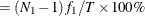 ) while Group 2 contributes 97%. Other measures like RMR, SRMR, and Bentler-Bonett NFI show that Group 1 data are fitted better.
The GFI’s show equal fits for the two groups, however.
) while Group 2 contributes 97%. Other measures like RMR, SRMR, and Bentler-Bonett NFI show that Group 1 data are fitted better.
The GFI’s show equal fits for the two groups, however.
Despite a very good fit, the current model is not intended to be the final model. It was fitted mainly for illustration purposes. The next section considers a partially constrained model for the two groups of data.
A Model with Partially Constrained Parameters for the Two Regions
For multiple-group analysis, cross-group constraints are of primary interest and should be explored whenever appropriate. The first fitting with all model parameters constrained for the groups has been shown to be too restrictive, while the current model with no cross-group constraints fits very well—so well that it might have overfit unnecessarily. A multiple-group model between these extremes is now explored. The following statements specify such a partially constrained model:
proc calis meanstr modification;
   group 1 / data=region1 label="Region 1" nobs=378;
   group 2 / data=region2 label="Region 2" nobs=423;
   model 3 / label="Model for References Only";
      path
         Service ===> Spend02  Spend03      ,
         Product ===> Spend02  Spend03      ,
         Spend02 ===> Spend03               ,
         Service ===> Courtesy Responsive
                      Helpful Delivery      ,
         Product ===> Pricing  Availability
                      Quality               ;
      pvar
         Courtesy Responsive Helpful Delivery Pricing
         Availability Quality Spend02 Spend03,
         Service Product = 2 * 1.;
      pcov
         Service Product;
   model 1 / groups=1;
      refmodel 3;
      mean
         Spend02 Spend03 = G1_InterSpend02 G1_InterSpend03,
         Courtesy Responsive Helpful
         Delivery Pricing Availability
         Quality = G1_intercept01-G1_intercept07;
   model 2 / groups=2;
      refmodel 3;
      mean
         Spend02 Spend03 = G2_InterSpend02 G2_InterSpend03,
         Courtesy Responsive Helpful
         Delivery Pricing Availability
         Quality = G2_intercept01-G2_intercept07;
      simtests
         SpendDiff       = (Spend02Diff Spend03Diff)
         MeasurementDiff = (CourtesyDiff ResponsiveDiff
                            HelpfulDiff DeliveryDiff
                            PricingDiff AvailabilityDiff
                            QualityDiff);
      Spend02Diff      = G2_InterSpend02 - G1_InterSpend02;
      Spend03Diff      = G2_InterSpend03 - G1_InterSpend03;
      CourtesyDiff     = G2_intercept01  - G1_intercept01;
      ResponsiveDiff   = G2_intercept02  - G1_intercept02;
      HelpfulDiff      = G2_intercept03  - G1_intercept03;
      DeliveryDiff     = G2_intercept04  - G1_intercept04;
      PricingDiff      = G2_intercept05  - G1_intercept05;
      AvailabilityDiff = G2_intercept06  - G1_intercept06;
      QualityDiff      = G2_intercept07  - G1_intercept07;
run;
In this specification, you use a special model definition. Model 3 serves as a reference model. You are not going to fit this model directly to any data set, but the specifications of other two models makes reference to it. Model 3 is no different from the basic path model specification used in preceding examples. The PATH model specification reflects the path diagram in Output 29.28.1.
Region 1 is fitted by Model 1, which makes reference to Model 3 by using the REFMODEL
statement. In addition, you add the MEAN statement specification. You now specify the intercept parameters explicitly by
using the parameter names G1_intercept01–G1_intercept07, G1_InterSpend02, and G1_InterSpend03. In previous examples, these intercept parameters are set by default by PROC CALIS. This explicit parameter naming serves
the purpose of distinguishing these parameters from those for Model 2.
Region 2 is fitted by Model 2, which also refers to Model 3 by using the REFMODEL
statement. You also specify a MEAN statement for this model with explicit specifications of the intercept parameters. You
name these intercepts G2_intercept01–G2_intercept07, G2_InterSpend02, and G2_InterSpend03. The G2 prefix distinguishes these parameters from the corresponding intercept parameters in the parent model. All in all, this means
that both Models 1 and 2 refers to Model 3, except that Model 2 uses a different set of intercept parameters. In other words,
in this multiple-group model the covariance structures for the two regions are constrained to be the same, while the means
structures are allowed to be unconstrained.
You request additional statistics or tests in the current PROC CALIS analysis. The MODIFICATION option in the PROC CALIS statement requests that the Lagrange multiplier tests and Wald tests be conducted. The Lagrange multiplier tests provide information about which constrained or fixed parameters could be freed or added so as to improve the overall model fit. The Wald tests provide information about which existing parameters could be fixed at zeros (eliminated) without significantly affecting the overall model fit. These tests are discussed in more detail when the results are presented.
In the SIMTESTS
statement, two simultaneous tests are requested. The first simultaneous test is named SpendDiff, which includes two parametric functions Spend02Diff and Spend03Diff. The second simultaneous test is named MeasurementDiff, which includes seven parametric functions: CourtesyDiff, ResponsiveDiff, HelpfulDiff, DeliveryDiff, PricingDiff, AvailabilityDiff, and QualityDiff. The null hypothesis of these simultaneous tests is of the form
![\[ H_0: t_ i = 0 \quad (i = 1 \ldots k) \]](images/statug_calis1063.png)
where k is the number of parametric functions within the simultaneous test. In the current analysis, the component parametric functions are defined in the SAS programming statements , which are shown in the last block of the specification. Essentially, all these parametric functions represent the differences of the mean or intercept parameters between the two models for groups. The first simultaneous test is intended to test whether the mean or intercept parameters in the structural models are the same, while the second simultaneous test is intended to test whether the mean parameters in the measurement models are the same.
The fit summary table is shown in Output 29.28.7.
Output 29.28.7: Fit Summary
| Fit Summary | ||
|---|---|---|
| Modeling Info | Number of Observations | 801 |
| Number of Variables | 9 | |
| Number of Moments | 108 | |
| Number of Parameters | 40 | |
| Number of Active Constraints | 0 | |
| Baseline Model Function Value | 0.5003 | |
| Baseline Model Chi-Square | 399.7468 | |
| Baseline Model Chi-Square DF | 72 | |
| Pr > Baseline Model Chi-Square | <.0001 | |
| Absolute Index | Fit Function | 0.1346 |
| Chi-Square | 107.5461 | |
| Chi-Square DF | 68 | |
| Pr > Chi-Square | 0.0016 | |
| Z-Test of Wilson & Hilferty | 2.9452 | |
| Hoelter Critical N | 657 | |
| Root Mean Square Residual (RMR) | 0.1577 | |
| Standardized RMR (SRMR) | 0.0678 | |
| Goodness of Fit Index (GFI) | 1.0000 | |
| Parsimony Index | Adjusted GFI (AGFI) | 0.9999 |
| Parsimonious GFI | 0.9444 | |
| RMSEA Estimate | 0.0382 | |
| RMSEA Lower 90% Confidence Limit | 0.0237 | |
| RMSEA Upper 90% Confidence Limit | 0.0514 | |
| Probability of Close Fit | 0.9275 | |
| Akaike Information Criterion | 187.5461 | |
| Bozdogan CAIC | 414.9806 | |
| Schwarz Bayesian Criterion | 374.9806 | |
| McDonald Centrality | 0.9756 | |
| Incremental Index | Bentler Comparative Fit Index | 0.8793 |
| Bentler-Bonett NFI | 0.7310 | |
| Bentler-Bonett Non-normed Index | 0.8722 | |
| Bollen Normed Index Rho1 | 0.7151 | |
| Bollen Non-normed Index Delta2 | 0.8808 | |
| James et al. Parsimonious NFI | 0.6904 | |
The chi-square value is 107.55 (df = 68, p = 0.0016), which is statistically significant. The null hypothesis of the mean and covariance structures is rejected if an
 -level at 0.01 or larger is chosen. However, in practical structural equation modeling, the chi-square test is not the only
criterion, or even an important criterion, for evaluating model fit. The RMSEA estimate for the current model is 0.0382, which
indicates a good fit. The probability level of close fit is 0.9275, indicating that a good population fit hypothesis (that
is, population RMSEA < 0.05) cannot be rejected. The GFI, AGFI, and parsimonious GFI all indicate good fit. However, the incremental
indices show only a respectable model fit.
-level at 0.01 or larger is chosen. However, in practical structural equation modeling, the chi-square test is not the only
criterion, or even an important criterion, for evaluating model fit. The RMSEA estimate for the current model is 0.0382, which
indicates a good fit. The probability level of close fit is 0.9275, indicating that a good population fit hypothesis (that
is, population RMSEA < 0.05) cannot be rejected. The GFI, AGFI, and parsimonious GFI all indicate good fit. However, the incremental
indices show only a respectable model fit.
Comparison of the model fit to the groups is shown in Output 29.28.8.
Output 29.28.8: Fit Comparison among Groups
| Fit Comparison Among Groups | ||||
|---|---|---|---|---|
| Overall | Region 1 | Region 2 | ||
| Modeling Info | Number of Observations | 801 | 378 | 423 |
| Number of Variables | 9 | 9 | 9 | |
| Number of Moments | 108 | 54 | 54 | |
| Number of Parameters | 40 | 31 | 31 | |
| Number of Active Constraints | 0 | 0 | 0 | |
| Baseline Model Function Value | 0.5003 | 0.4601 | 0.5363 | |
| Baseline Model Chi-Square | 399.7468 | 173.4482 | 226.2986 | |
| Baseline Model Chi-Square DF | 72 | 36 | 36 | |
| Fit Index | Fit Function | 0.1346 | 0.1261 | 0.1422 |
| Percent Contribution to Chi-Square | 100 | 44 | 56 | |
| Root Mean Square Residual (RMR) | 0.1577 | 0.1552 | 0.1599 | |
| Standardized RMR (SRMR) | 0.0678 | 0.0792 | 0.0557 | |
| Goodness of Fit Index (GFI) | 1.0000 | 1.0000 | 1.0000 | |
| Bentler-Bonett NFI | 0.7310 | 0.7260 | 0.7348 | |
Looking at the percentage contribution to the chi-square, the Region 2 fitting shows a worse fit. However, this might be due to the larger sample size in Region 2. When comparing the fit of the two regions by using RMR, which does not take the sample size into account, the fitting of two groups are about the same. The standardized RMR even shows that Region 2 is fitted better. So, it seems to be safe to conclude that the models fit almost equally well (or badly) for the two regions.
The constrained parameter estimates for the two regions are shown in Output 29.28.9.
Output 29.28.9: Estimates of Path Coefficients and Other Covariance Parameters
| Model 1. PATH List | |||||||
|---|---|---|---|---|---|---|---|
| Path | Parameter | Estimate | Standard Error |
t Value | Pr > |t| | ||
| Service | ===> | Spend02 | _Parm01 | 0.37475 | 0.21318 | 1.7579 | 0.0788 |
| Service | ===> | Spend03 | _Parm02 | 0.53851 | 0.20840 | 2.5840 | 0.0098 |
| Product | ===> | Spend02 | _Parm03 | 0.80372 | 0.21939 | 3.6635 | 0.0002 |
| Product | ===> | Spend03 | _Parm04 | 0.59879 | 0.22144 | 2.7041 | 0.0068 |
| Spend02 | ===> | Spend03 | _Parm05 | 0.08952 | 0.03694 | 2.4233 | 0.0154 |
| Service | ===> | Courtesy | _Parm06 | 0.72418 | 0.07989 | 9.0648 | <.0001 |
| Service | ===> | Responsive | _Parm07 | 0.90452 | 0.08886 | 10.1797 | <.0001 |
| Service | ===> | Helpful | _Parm08 | 0.64969 | 0.07683 | 8.4557 | <.0001 |
| Service | ===> | Delivery | _Parm09 | 0.64473 | 0.09021 | 7.1468 | <.0001 |
| Product | ===> | Pricing | _Parm10 | 0.63452 | 0.07916 | 8.0160 | <.0001 |
| Product | ===> | Availability | _Parm11 | 0.76737 | 0.08265 | 9.2852 | <.0001 |
| Product | ===> | Quality | _Parm12 | 0.79716 | 0.08922 | 8.9347 | <.0001 |
| Model 1. Variance Parameters | ||||||
|---|---|---|---|---|---|---|
| Variance Type |
Variable | Parameter | Estimate | Standard Error |
t Value | Pr > |t| |
| Error | Courtesy | _Parm13 | 1.98374 | 0.13169 | 15.0638 | <.0001 |
| Responsive | _Parm14 | 2.02152 | 0.16159 | 12.5101 | <.0001 | |
| Helpful | _Parm15 | 1.96535 | 0.12263 | 16.0273 | <.0001 | |
| Delivery | _Parm16 | 2.97542 | 0.17049 | 17.4518 | <.0001 | |
| Pricing | _Parm17 | 1.93952 | 0.12326 | 15.7358 | <.0001 | |
| Availability | _Parm18 | 1.63156 | 0.13067 | 12.4865 | <.0001 | |
| Quality | _Parm19 | 2.08849 | 0.15329 | 13.6246 | <.0001 | |
| Spend02 | _Parm20 | 13.47066 | 0.71842 | 18.7505 | <.0001 | |
| Spend03 | _Parm21 | 13.02883 | 0.68682 | 18.9697 | <.0001 | |
| Exogenous | Service | 1.00000 | ||||
| Product | 1.00000 | |||||
All parameter estimates but one are statistically significant at  . The parameter
 _Parm01, which represents the path coefficient from Service to Spend02, has a t value of 1.76. This is only marginally significant. Although all these results bear the title of Model 1, these estimates
are the same for Model 2, of which the corresponding results are not shown here.
The mean and intercept parameters for the two models (regions) are shown in Output 29.28.10.
Output 29.28.10: Estimates of Means and Intercepts
| Model 1. Means and Intercepts | ||||||
|---|---|---|---|---|---|---|
| Type | Variable | Parameter | Estimate | Standard Error |
t Value | Pr > |t| |
| Intercept | Spend02 | G1_InterSpend02 | 183.50000 | 0.19585 | 937.0 | <.0001 |
| Spend03 | G1_InterSpend03 | 285.49480 | 6.78127 | 42.1005 | <.0001 | |
| Courtesy | G1_intercept01 | 4.31200 | 0.08157 | 52.8652 | <.0001 | |
| Responsive | G1_intercept02 | 4.72400 | 0.08679 | 54.4310 | <.0001 | |
| Helpful | G1_intercept03 | 3.92100 | 0.07958 | 49.2720 | <.0001 | |
| Delivery | G1_intercept04 | 4.35700 | 0.09484 | 45.9397 | <.0001 | |
| Pricing | G1_intercept05 | 6.14400 | 0.07882 | 77.9499 | <.0001 | |
| Availability | G1_intercept06 | 4.99400 | 0.07674 | 65.0732 | <.0001 | |
| Quality | G1_intercept07 | 5.97100 | 0.08500 | 70.2454 | <.0001 | |
| Model 2. Means and Intercepts | ||||||
|---|---|---|---|---|---|---|
| Type | Variable | Parameter | Estimate | Standard Error |
t Value | Pr > |t| |
| Intercept | Spend02 | G2_InterSpend02 | 156.25000 | 0.18511 | 844.1 | <.0001 |
| Spend03 | G2_InterSpend03 | 299.68311 | 5.77478 | 51.8952 | <.0001 | |
| Courtesy | G2_intercept01 | 2.41200 | 0.07709 | 31.2863 | <.0001 | |
| Responsive | G2_intercept02 | 2.72700 | 0.08203 | 33.2435 | <.0001 | |
| Helpful | G2_intercept03 | 5.22400 | 0.07522 | 69.4532 | <.0001 | |
| Delivery | G2_intercept04 | 6.37600 | 0.08964 | 71.1270 | <.0001 | |
| Pricing | G2_intercept05 | 7.14700 | 0.07450 | 95.9343 | <.0001 | |
| Availability | G2_intercept06 | 3.23300 | 0.07254 | 44.5702 | <.0001 | |
| Quality | G2_intercept07 | 5.11900 | 0.08034 | 63.7150 | <.0001 | |
All the mean and intercept estimates are statistically significant at  . Except for the fixed zero means for
 Service and Product, a quick glimpse of these mean and intercepts estimates shows a quite different pattern for the two models. Do these estimates
truly differ beyond chance? The simultaneous tests of these parameter estimates shown in Output 29.28.11 can confirm this.
Output 29.28.11 shows two simultaneous tests, as requested in the original statements.
Output 29.28.11: Simultaneous Tests
| Simultaneous Tests | |||||
|---|---|---|---|---|---|
| Simultaneous Test |
Parametric Function |
Function Value |
DF | Chi-Square | p Value |
| SpendDiff | 2 | 10458 | <.0001 | ||
| Spend02Diff | -27.25000 | 1 | 10225 | <.0001 | |
| Spend03Diff | 14.18831 | 1 | 185.86725 | <.0001 | |
| MeasurementDiff | 7 | 1610 | <.0001 | ||
| CourtesyDiff | -1.90000 | 1 | 286.58605 | <.0001 | |
| ResponsiveDiff | -1.99700 | 1 | 279.63659 | <.0001 | |
| HelpfulDiff | 1.30300 | 1 | 141.59942 | <.0001 | |
| DeliveryDiff | 2.01900 | 1 | 239.35318 | <.0001 | |
| PricingDiff | 1.00300 | 1 | 85.52567 | <.0001 | |
| AvailabilityDiff | -1.76100 | 1 | 278.09360 | <.0001 | |
| QualityDiff | -0.85200 | 1 | 53.06240 | <.0001 | |
The first one is SpendDiff, which tests simultaneously the following hypotheses:
 : G2_InterSpend02 = G1_InterSpend02
: G2_InterSpend03 = G1_InterSpend03
The exceedingly large chi-square value 10,460 suggests the composite null hypothesis is false. Individual tests for these hypotheses suggest that each of these hypotheses should be rejected. The chi-square values for individual tests are 10,227 and 185.84, respectively.
Similarly, the simultaneous and individual tests of the intercepts in the measurement model suggest that the two models (groups)
differ significantly in the means of the measured variables. Region 2 has significantly higher means in variables Helpful, Delivery, and Pricing, but significantly lower means in variables Courtesy, Responsive, Availability, and Quality.
Now you are ready to answer the main research questions. The overall customer service (Service) does affect the future purchase (Spend03), but not the current purchase (Spend02), because the corresponding path coefficient (_Parm01) is only marginally significant. Perhaps this is an artifact because the rating was done after the purchases in 2002. That
is, purchases in 2002 had been done before the impression about customer service was fully formed. However, this argument
cannot explain why overall customer service (Service) also shows a strong and significant relationship with purchases in 2002 (Spend02). Nonetheless, customer service and product quality do affect the future purchases (Spend03) in an expected way, even after partialling out the effect of the previous purchase amount (Spend02). Apart from the mean differences of the variables, the common measurement and prediction (or structural) models fit the
two regions very well.
Because the current model fits well and most parts of fitting meet your expectations, you might accept this model without looking for further improvement. Nonetheless, for illustration purposes, it would be useful to consider the LM test results. In Output 29.28.12, ranked LM statistics for the path coefficients in Model 1 and Model 2 are shown.
Output 29.28.12: LM Tests for Path Coefficients
| Model 1. Rank Order of the 10 Largest LM Stat for Path Relations | ||||
|---|---|---|---|---|
| To | From | LM Stat | Pr > ChiSq | Parm Change |
| Service | Courtesy | 11.15249 | 0.0008 | -0.17145 |
| Service | Helpful | 3.09038 | 0.0788 | 0.09431 |
| Service | Delivery | 2.59511 | 0.1072 | 0.07504 |
| Courtesy | Responsive | 1.75943 | 0.1847 | -0.07730 |
| Delivery | Courtesy | 1.66721 | 0.1966 | 0.08669 |
| Helpful | Courtesy | 1.62005 | 0.2031 | 0.07277 |
| Courtesy | Product | 1.48928 | 0.2223 | -0.14815 |
| Service | Product | 0.83498 | 0.3608 | -0.12327 |
| Responsive | Helpful | 0.76664 | 0.3813 | -0.05625 |
| Product | Helpful | 0.53020 | 0.4665 | -0.03831 |
| Model 2. Rank Order of the 10 Largest LM Stat for Path Relations | ||||
|---|---|---|---|---|
| To | From | LM Stat | Pr > ChiSq | Parm Change |
| Delivery | Courtesy | 16.91167 | <.0001 | -0.26641 |
| Service | Courtesy | 9.11235 | 0.0025 | 0.15430 |
| Courtesy | Delivery | 8.12091 | 0.0044 | -0.12989 |
| Courtesy | Responsive | 8.03954 | 0.0046 | 0.16215 |
| Pricing | Responsive | 5.48406 | 0.0192 | 0.10424 |
| Courtesy | Product | 4.39347 | 0.0361 | 0.24412 |
| Courtesy | Quality | 3.52147 | 0.0606 | 0.08672 |
| Service | Delivery | 3.20160 | 0.0736 | -0.08281 |
| Service | Helpful | 2.97015 | 0.0848 | -0.09198 |
| Responsive | Pricing | 2.91498 | 0.0878 | 0.08943 |
Path coefficients that lead to better improvement (larger chi-square decrease) are shown first in the tables. For example,
the first path coefficient that is suggested to be freed in Model 1 is the Service <=== Courtesy path. The associated p-value is 0.0008 and the estimated change of parameter value is –0.171. The second path coefficient is for the Service <=== Helpful path, but it is not significant at the 0.05 level. So, is it good to add the Service <=== Courtesy path to Model 1, based on the LM test results? The answer is that it depends on your application and the theoretical and
practical implications. For example, the Service ===> Courtesy path, which is a part of the measurement model, is already specified in Model 1. Even though the LM test statistic shows
a significant decrease of model fit chi-square, adding the Service <=== Courtesy path might destroy the measurement model and lead to problematic interpretations. In this case, it is wise not to add the
Service <=== Courtesy path, which is suggested by the LM test results.
LM tests for the path coefficients in Model 2 are shown at the bottom of Output 29.28.12. Quite a few of these tests suggest significant improvements in model fit. Again, you are cautioned against adding these paths blindly.
LM tests for the error variances and covariances are shown in Output 29.28.13.
Output 29.28.13: LM Tests for Error Covariances
| Model 1. Rank Order of the 10 Largest LM Stat for Error Variances and Covariances | ||||
|---|---|---|---|---|
| Error of |
Error of |
LM Stat | Pr > ChiSq | Parm Change |
| Responsive | Helpful | 1.26589 | 0.2605 | -0.15774 |
| Delivery | Courtesy | 0.70230 | 0.4020 | 0.12577 |
| Helpful | Courtesy | 0.50167 | 0.4788 | 0.09103 |
| Quality | Availability | 0.47993 | 0.4885 | -0.09739 |
| Quality | Pricing | 0.45925 | 0.4980 | 0.09449 |
| Responsive | Availability | 0.25734 | 0.6120 | 0.05965 |
| Helpful | Availability | 0.24811 | 0.6184 | -0.05413 |
| Responsive | Pricing | 0.23748 | 0.6260 | -0.05911 |
| Spend02 | Availability | 0.19634 | 0.6577 | -0.13200 |
| Responsive | Courtesy | 0.18212 | 0.6696 | 0.06201 |
| Model 2. Rank Order of the 10 Largest LM Stat for Error Variances and Covariances | ||||
|---|---|---|---|---|
| Error of |
Error of |
LM Stat | Pr > ChiSq | Parm Change |
| Delivery | Courtesy | 16.00996 | <.0001 | -0.57408 |
| Responsive | Pricing | 4.89190 | 0.0270 | 0.25403 |
| Helpful | Delivery | 3.33480 | 0.0678 | 0.25299 |
| Delivery | Availability | 2.79513 | 0.0946 | 0.20656 |
| Responsive | Availability | 2.16944 | 0.1408 | -0.16421 |
| Quality | Courtesy | 2.14952 | 0.1426 | 0.17094 |
| Responsive | Courtesy | 2.12832 | 0.1446 | 0.20604 |
| Quality | Pricing | 2.00978 | 0.1563 | -0.19154 |
| Quality | Availability | 1.99477 | 0.1578 | 0.19459 |
| Responsive | Quality | 1.88736 | 0.1695 | -0.16963 |
Using , you might consider adding two pairs of correlated errors in Model 2. The first pair is for Delivery and Courtesy, which has a p-value less than 0.0001. The second pair is Pricing and Responsive, which has a p-value of 0.027. Again, adding correlated errors (in the PCOV
statement) should not be a pure statistical consideration. You should also consider theoretical and practical implications.
LM tests for other subsets of parameters are also conducted. Some subsets do not have parameters that can be freed, and so they are not shown here. Other subsets are not shown here simply for conserving space.
PROC CALIS ranks and outputs the LM test results for some default subsets of parameters. You have seen the subsets for path coefficients and correlated errors in the two previous outputs. Some other LM test results are not shown. With this kind of default LM output, there could be a huge amount of modification indices to look at. Fortunately, you can limit the LM test results to any subsets of potential parameters that you might be interested in. With your substantive knowledge, you can define such meaningful subsets of potential parameters by using the LMTESTS statement. The LM test indices and rankings are then done for each predefined subset of potential parameters. With these customized LM results, you can limit your attention to consider only those meaningful parameters to be added. See the LMTESTS statement for details.
The next group of LM tests is for releasing implicit equality constraints in your model, as shown in Output 29.28.14.
Output 29.28.14: LM Tests for Equality Constraints
| Lagrange Multiplier Statistics for Releasing Equality Constraints | ||||||||
|---|---|---|---|---|---|---|---|---|
| Parm | Released Parameter | LM Stat | Pr > ChiSq | Changes | ||||
|
Model |
Type |
Var1 | Var2 | Original Parm |
Released Parm |
|||
| _Parm01 | 1 | DV_IV | Spend02 | Service | 0.01554 | 0.9008 | -0.0213 | 0.0238 |
| 2 | DV_IV | Spend02 | Service | 0.01554 | 0.9008 | 0.0238 | -0.0213 | |
| _Parm02 | 1 | DV_IV | Spend03 | Service | 0.01763 | 0.8944 | -0.0222 | 0.0248 |
| 2 | DV_IV | Spend03 | Service | 0.01763 | 0.8944 | 0.0248 | -0.0222 | |
| _Parm03 | 1 | DV_IV | Spend02 | Product | 0.0003403 | 0.9853 | -0.00321 | 0.00355 |
| 2 | DV_IV | Spend02 | Product | 0.0003403 | 0.9853 | 0.00355 | -0.00321 | |
| _Parm04 | 1 | DV_IV | Spend03 | Product | 0.00176 | 0.9665 | 0.00714 | -0.00802 |
| 2 | DV_IV | Spend03 | Product | 0.00176 | 0.9665 | -0.00802 | 0.00714 | |
| _Parm05 | 1 | DV_DV | Spend03 | Spend02 | 0.0009698 | 0.9752 | -0.00100 | 0.00112 |
| 2 | DV_DV | Spend03 | Spend02 | 0.0009698 | 0.9752 | 0.00112 | -0.00100 | |
| _Parm06 | 1 | DV_IV | Courtesy | Service | 19.17225 | <.0001 | 0.2851 | -0.3191 |
| 2 | DV_IV | Courtesy | Service | 19.17225 | <.0001 | -0.3191 | 0.2851 | |
| _Parm07 | 1 | DV_IV | Responsive | Service | 0.21266 | 0.6447 | -0.0304 | 0.0341 |
| 2 | DV_IV | Responsive | Service | 0.21266 | 0.6447 | 0.0341 | -0.0304 | |
| _Parm08 | 1 | DV_IV | Helpful | Service | 4.60629 | 0.0319 | -0.1389 | 0.1555 |
| 2 | DV_IV | Helpful | Service | 4.60629 | 0.0319 | 0.1555 | -0.1389 | |
| _Parm09 | 1 | DV_IV | Delivery | Service | 3.59763 | 0.0579 | -0.1508 | 0.1687 |
| 2 | DV_IV | Delivery | Service | 3.59763 | 0.0579 | 0.1687 | -0.1508 | |
| _Parm10 | 1 | DV_IV | Pricing | Product | 0.50974 | 0.4753 | 0.0468 | -0.0524 |
| 2 | DV_IV | Pricing | Product | 0.50974 | 0.4753 | -0.0524 | 0.0468 | |
| _Parm11 | 1 | DV_IV | Availability | Product | 0.57701 | 0.4475 | -0.0457 | 0.0512 |
| 2 | DV_IV | Availability | Product | 0.57701 | 0.4475 | 0.0512 | -0.0457 | |
| _Parm12 | 1 | DV_IV | Quality | Product | 0.00566 | 0.9400 | -0.00511 | 0.00574 |
| 2 | DV_IV | Quality | Product | 0.00566 | 0.9400 | 0.00574 | -0.00511 | |
| _Parm13 | 1 | COVERR | Courtesy | Courtesy | 45.24725 | <.0001 | 0.7204 | -0.8064 |
| 2 | COVERR | Courtesy | Courtesy | 45.24725 | <.0001 | -0.8064 | 0.7204 | |
| _Parm14 | 1 | COVERR | Responsive | Responsive | 1.73499 | 0.1878 | -0.1555 | 0.1740 |
| 2 | COVERR | Responsive | Responsive | 1.73499 | 0.1878 | 0.1740 | -0.1555 | |
| _Parm15 | 1 | COVERR | Helpful | Helpful | 11.13266 | 0.0008 | -0.3448 | 0.3860 |
| 2 | COVERR | Helpful | Helpful | 11.13266 | 0.0008 | 0.3860 | -0.3448 | |
| _Parm16 | 1 | COVERR | Delivery | Delivery | 4.99097 | 0.0255 | -0.3364 | 0.3766 |
| 2 | COVERR | Delivery | Delivery | 4.99097 | 0.0255 | 0.3766 | -0.3364 | |
| _Parm17 | 1 | COVERR | Pricing | Pricing | 2.86428 | 0.0906 | 0.1729 | -0.1936 |
| 2 | COVERR | Pricing | Pricing | 2.86428 | 0.0906 | -0.1936 | 0.1729 | |
| _Parm18 | 1 | COVERR | Availability | Availability | 2.53147 | 0.1116 | -0.1494 | 0.1672 |
| 2 | COVERR | Availability | Availability | 2.53147 | 0.1116 | 0.1672 | -0.1494 | |
| _Parm19 | 1 | COVERR | Quality | Quality | 0.07328 | 0.7866 | -0.0315 | 0.0352 |
| 2 | COVERR | Quality | Quality | 0.07328 | 0.7866 | 0.0352 | -0.0315 | |
| _Parm20 | 1 | COVERR | Spend02 | Spend02 | 0.00214 | 0.9631 | 0.0304 | -0.0340 |
| 2 | COVERR | Spend02 | Spend02 | 0.00214 | 0.9631 | -0.0340 | 0.0304 | |
| _Parm21 | 1 | COVERR | Spend03 | Spend03 | 0.0001773 | 0.9894 | -0.00842 | 0.00946 |
| 2 | COVERR | Spend03 | Spend03 | 0.0001773 | 0.9894 | 0.00946 | -0.00842 | |
| _Parm22 | 1 | COVEXOG | Service | Product | 0.87147 | 0.3505 | 0.0605 | -0.0678 |
| 2 | COVEXOG | Service | Product | 0.87147 | 0.3505 | -0.0678 | 0.0605 | |
Recall that the measurement and the prediction models for the two regions are constrained to be the same by model referencing
(that is, the REFMODEL
statement). Output 29.28.14 shows you which parameter can be unconstrained so that your overall model fit might improve. For example, if you unconstrain
the first parameter _Parm01, which is for the path effect of Spend02 <=== Service, for the two models, the expected chi-square decrease (LM Stat) is about 0.0158, which is not significant (p = .9001). The associated parameter changes are small too. However, if you consider unconstraining parameter _Parm06, which is for the path effect of Courtesy <=== Service, the expected decrease of chi-square is 19.22 ( ). There are two rows for this parameter. Each row represents a parameter location to be released from the equality constraint.
Consider the first row first. If you rename the coefficient for the
). There are two rows for this parameter. Each row represents a parameter location to be released from the equality constraint.
Consider the first row first. If you rename the coefficient for the Courtesy <=== Service path in Model 1 to a new parameter, say "new" (while keeping _Parm06 as the parameter for the Courtesy <=== Service path in Model 2) and fit the model again, the new estimate of _Parm06 is 0.2852 greater than the previous _Parm06 estimate. The estimate of "new" is 0.3196 less than the previous _Parm06 estimate. The second row for the _Parm06 parameter shows similar but reflected results. It is for renaming the parameter location in Model 2. For this example each
equality constraint has exactly two locations, one for Model 1 and one for Model 2. That is the reason why you always observe
reflected results for freeing the locations successively. Reflected results are not the case if you have equality constraints
with more than two parameter locations.
Another example of a large expected improvement of model fit is the result of freeing the constrained variances of Courtesy among the two models. The corresponding row to look at is the row with parameter _Parm13, where the parameter type is labeled "COVERR" and the values for Var1 and Var2 are both "Courtesy." The LM statistic is 45.255, which is a significant chi-square decrease if you free either parameter
location. If you choose to rename the error variance for Courtesy in Model 1, the new _Parm13 estimate is 0.8052 smaller than the original _Parm13 estimate. The new estimate of the error variance for Courtesy in Model 2 is 0.7211 greater than the previous _Parm13 estimate. Finally, the constrained parameter _Parm15, which is the error variance parameter for Helpful in both models, is also a potential constraint that can be released with a significant model fit improvement.
In addition to the LM statistics for suggesting ways to improve model fit, PROC CALIS also computes the Wald tests to show which parameters can be constrained to zero without jeopardizing the model fit significantly. The Wald test results are shown in Output 29.28.15.
Output 29.28.15: Wald Tests
In Output 29.28.15, you see that _Parm01, which is for the path effect of Spend02 <=== Service, is suggested to be a fixed zero parameter (eliminated from the model) by the Wald test. Fixing this parameter to zero (or
dropping the Spend02 <=== Service path from the model) is expected to increase the model fit chi-square by 3.085 (p = .079), which is only marginally significant at .
As is the case for the LM test statistics, you should not automatically adhere to the suggestions by the Wald statistics. Substantive and theoretical considerations should always be considered when determining whether a parameter should be added or dropped.