The CALIS Procedure
-
Overview

-
Getting Started
-
SyntaxClasses of Statements in PROC CALISSingle-Group Analysis SyntaxMultiple-Group Multiple-Model Analysis SyntaxPROC CALIS StatementBOUNDS StatementBY StatementCOSAN StatementCOV StatementDETERM StatementEFFPART StatementFACTOR StatementFITINDEX StatementFREQ StatementGROUP StatementLINCON StatementLINEQS StatementLISMOD StatementLMTESTS StatementMATRIX StatementMEAN StatementMODEL StatementMSTRUCT StatementNLINCON StatementNLOPTIONS StatementOUTFILES StatementPARAMETERS StatementPARTIAL StatementPATH StatementPATHDIAGRAM StatementPCOV StatementPVAR StatementRAM StatementREFMODEL StatementRENAMEPARM StatementSAS Programming StatementsSIMTESTS StatementSTD StatementSTRUCTEQ StatementTESTFUNC StatementVAR StatementVARIANCE StatementVARNAMES StatementWEIGHT Statement
-
DetailsInput Data SetsOutput Data SetsDefault Analysis Type and Default ParameterizationThe COSAN ModelThe FACTOR ModelThe LINEQS ModelThe LISMOD Model and SubmodelsThe MSTRUCT ModelThe PATH ModelThe RAM ModelNaming Variables and ParametersSetting Constraints on ParametersAutomatic Variable SelectionPath Diagrams: Layout Algorithms, Default Settings, and CustomizationEstimation CriteriaRelationships among Estimation CriteriaGradient, Hessian, Information Matrix, and Approximate Standard ErrorsCounting the Degrees of FreedomAssessment of FitCase-Level Residuals, Outliers, Leverage Observations, and Residual DiagnosticsLatent Variable ScoresTotal, Direct, and Indirect EffectsStandardized SolutionsModification IndicesMissing Values and the Analysis of Missing PatternsMeasures of Multivariate KurtosisInitial EstimatesUse of Optimization TechniquesComputational ProblemsDisplayed OutputODS Table NamesODS Graphics
-
ExamplesEstimating Covariances and CorrelationsEstimating Covariances and Means SimultaneouslyTesting Uncorrelatedness of VariablesTesting Covariance PatternsTesting Some Standard Covariance Pattern HypothesesLinear Regression ModelMultivariate Regression ModelsMeasurement Error ModelsTesting Specific Measurement Error ModelsMeasurement Error Models with Multiple PredictorsMeasurement Error Models Specified As Linear EquationsConfirmatory Factor ModelsConfirmatory Factor Models: Some VariationsResidual Diagnostics and Robust EstimationThe Full Information Maximum Likelihood MethodComparing the ML and FIML EstimationPath Analysis: Stability of AlienationSimultaneous Equations with Mean Structures and Reciprocal PathsFitting Direct Covariance StructuresConfirmatory Factor Analysis: Cognitive AbilitiesTesting Equality of Two Covariance Matrices Using a Multiple-Group AnalysisTesting Equality of Covariance and Mean Matrices between Independent GroupsIllustrating Various General Modeling LanguagesTesting Competing Path Models for the Career Aspiration DataFitting a Latent Growth Curve ModelHigher-Order and Hierarchical Factor ModelsLinear Relations among Factor LoadingsMultiple-Group Model for Purchasing BehaviorFitting the RAM and EQS Models by the COSAN Modeling LanguageSecond-Order Confirmatory Factor AnalysisLinear Relations among Factor Loadings: COSAN Model SpecificationOrdinal Relations among Factor LoadingsLongitudinal Factor Analysis
- References
Example 29.17 Path Analysis: Stability of Alienation
The following covariance matrix from Wheaton et al. (1977) has served to illustrate the performance of several implementations for the analysis of structural equation models. Two different models have been analyzed by an early implementation of LISREL and are mentioned in Jöreskog (1978). You can also find a more detailed discussion of these models in the LISREL VI manual (Jöreskog and Sörbom 1985). A slightly modified model for this covariance matrix is included in the EQS 2.0 manual (Bentler 1985, p. 28). However, for the analysis with the EQS implementation, the SEI variable is rescaled by a factor of 0.1 to make the matrix less ill-conditioned. Since the Levenberg-Marquardt or Newton-Raphson optimization techniques are used with PROC CALIS, rescaling the data matrix is not necessary and, therefore, is not done here. The results reported here reflect the estimates based on the original covariance matrix.
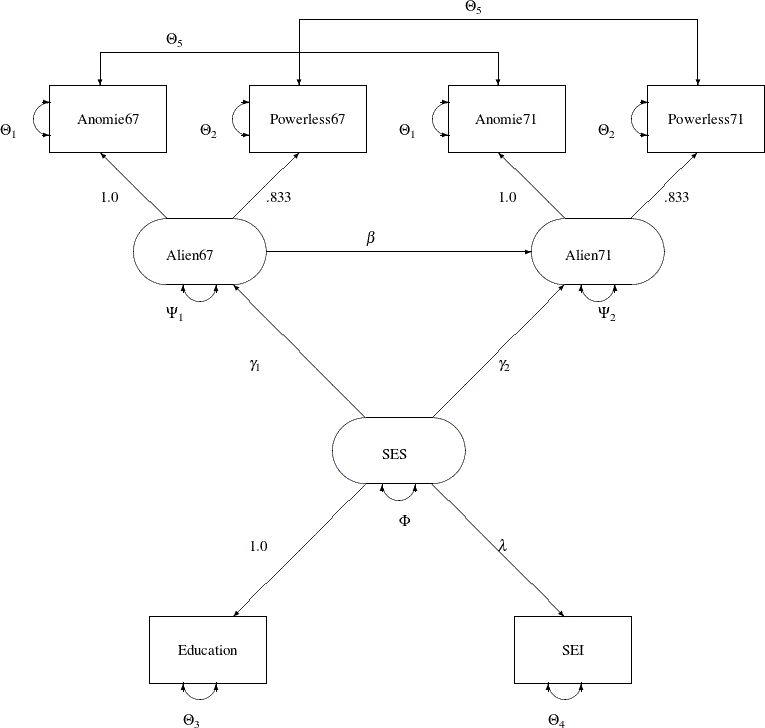
The path diagram of this model is displayed in Figure 29.1 and is reproduced in the following:
Output 29.17.1:
You use the PATH modeling language of PROC CALIS to specify this path model, as shown in the following statements:
title "Stability of Alienation";
title2 "Data Matrix of WHEATON, MUTHEN, ALWIN & SUMMERS (1977)";
data Wheaton(TYPE=COV);
   _type_ = 'cov';
   input _name_ $ 1-11 Anomie67 Powerless67 Anomie71 Powerless71
                       Education SEI;
   label Anomie67='Anomie (1967)' Powerless67='Powerlessness (1967)'
         Anomie71='Anomie (1971)' Powerless71='Powerlessness (1971)'
         Education='Education'    SEI='Occupational Status Index';
   datalines;
Anomie67       11.834     .        .        .       .        .
Powerless67     6.947    9.364     .        .       .        .
Anomie71        6.819    5.091   12.532     .       .        .
Powerless71     4.783    5.028    7.495    9.986    .        .
Education      -3.839   -3.889   -3.841   -3.625   9.610     .
SEI           -21.899  -18.831  -21.748  -18.775  35.522  450.288
;
ods graphics on;

proc calis nobs=932 data=Wheaton plots=residuals;
   path
      Anomie67   Powerless67  <===  Alien67   = 1.0  0.833,
      Anomie71   Powerless71  <===  Alien71   = 1.0  0.833,
      Education  SEI          <===  SES       = 1.0  lambda,
      Alien67    Alien71      <===  SES       = gamma1 gamma2,
      Alien71                 <===  Alien67   = beta;
   pvar
      Anomie67     = theta1,
      Powerless67  = theta2,
      Anomie71     = theta1,
      Powerless71  = theta2,
      Education    = theta3,
      SEI          = theta4,
      Alien67      = psi1,
      Alien71      = psi2,
      SES          = phi;
   pcov
      Anomie67    Anomie71    = theta5,
      Powerless67 Powerless71 = theta5;
   pathdiagram title='Stability of Alienation';
run;

ods graphics off;
Since no METHOD= option is used in the PROC CALIS statement, maximum likelihood estimates are computed by default.
In the PATH statement, you specify the functional relationships of the variables in the model. These functional relationships
are represented as single-headed paths in the path diagram. There are five entries in the PATH statement. You specify the
relationships between the latent constructs and the observed variables in the first three path entries. For example, the first
entry states that Anomie and Powerless67 are measured indicators of the latent variable Alien67. The path effects or coefficients from the latent factor to these measured indicators are fixed at 1.0 and 0.833, respectively.
Similarly, in the next two path entries, you define the relationships between the latent factors Alien71 and SES and their measured indicators. The last two path entries in the PATH statement represent the functional relationships among
the latent variables in the model. SES has effects on Alien67 and Alien71. These effect parameters are labeled or named with gamma1 and gamma2, respectively. Alien67 also has an effect on Alien71, with the effect parameter named beta.
In the PVAR statement, you specify the variance or error variance parameters in the model. These parameters correspond to
the double-headed arrows pointing to the individual variables in the path diagram. In the first six entries of the PVAR statement,
you specify the error variance parameters of the observed variables. You also give names to these parameters that correspond
to the notation in the path diagram. Although you can choose any names for the parameters, it is important to remember that
parameters with the same name are identical and will have the same estimates. For example, the error variances of Anomie67 and Anomie71 are the same parameter named theta1. Similarly, you constrain the error variances of Powerless67 and Powerless71. However, the error variance parameters of Education and SEI are unique. They are not constrained with other parameters in the model because they have unique parameter names. Next, you
specify the error variance parameters of Alien67 and Alien71. They also have unique parameter names and therefore they are not constrained with any other parameters in the model. Lastly,
you specify the variance parameter phi of SES.
In the PCOV statement, you specify the covariances or error covariances among variables in the model. These parameters correspond
to the double-headed arrows pointing to distinct pairs of variables in the path diagram. Observed variables Anomie67 and Anomie71 have correlated errors and you specify this error covariance parameter as theta5. Similarly, observed variables Powerless67 and Powerless71 have correlated errors and you also specify this error covariance parameter as theta5. This way, the two error covariances are constrained to be equal.
PROC CALIS can produce a high-quality residual histogram that is useful for showing the distribution of residuals. Before
you request the residual histogram, ODS Graphics must be enabled. For example, you can specify the ODS GRAPHICS ON statement,
as shown in the preceding statements before the PROC CALIS statement. Then, the residual histogram is requested by the plots=residuals option in the PROC CALIS statement. PROC CALIS can also produce a high-quality path diagram for the model. You can use the
PATHDIAGRAM statement to request the path diagram and to specify related options.
Output 29.17.2 displays the modeling information and variables in the analysis.
Output 29.17.2: Model Specification and Variables
Output 29.17.2 shows that the data set Wheaton was used with 932 observations. The model is specified with the PATH modeling language. Variables in the model are classified
into different categories according to their roles. All manifest variables are endogenous in the model. Also, three latent
variables are hypothesized in the model: Alien67, Alien71, and SES. While Alien67 and Alien71 are endogenous, SES is exogenous in the model.
Output 29.17.3 echoes the initial specification of the PATH model.
Output 29.17.3: Initial Estimates
| Initial Estimates for PATH List | ||||
|---|---|---|---|---|
| Path | Parameter | Estimate | ||
| Anomie67 | <=== | Alien67 | 1.00000 | |
| Powerless67 | <=== | Alien67 | 0.83300 | |
| Anomie71 | <=== | Alien71 | 1.00000 | |
| Powerless71 | <=== | Alien71 | 0.83300 | |
| Education | <=== | SES | 1.00000 | |
| SEI | <=== | SES | lambda | . |
| Alien67 | <=== | SES | gamma1 | . |
| Alien71 | <=== | SES | gamma2 | . |
| Alien71 | <=== | Alien67 | beta | . |
The numerical values for estimates in Output 29.17.3 are the initial values that you input in the model specification. A blank value for the associated parameter name for a numerical
estimate indicates that the estimate is a fixed value, which would not be changed in the estimation. For example, the first
five paths have fixed path coefficients, and their fixed values are shown in the Estimate column. For numerical estimates
that have specified parameter names, the numerical values serve as initial values, which would be changed during the estimation.
Output 29.17.3 does not actually have this type of specification. Missing values '.' are specified as initial values for all the free parameters
that are specified in the model. For example, lambda, gamma1, theta1, and psi1, among others, are free parameters that do not have specified initial values. PROC CALIS automatically generates the initial
values of these parameters.
You can examine this output to ensure that the desired model is being analyzed. PROC CALIS outputs the initial specifications or the estimation results in the order you specify in the model, unless you use reordering options such as ORDERSPEC and ORDERALL . Therefore, the input order of specifications is important—it determines how your output would look.
Simple descriptive statistics are displayed in Output 29.17.4.
Output 29.17.4: Descriptive Statistics
Because the input data set contains only the covariance matrix, the means of the manifest variables are assumed to be zero.
Note that this has no impact on the estimation, unless a mean structure model is being analyzed.
Initial estimates are necessary in all kinds of optimization problems. You can provide these initial estimates or let PROC CALIS to generate them automatically. As shown in Output 29.17.3, you did not provide any initial estimates for the parameters. PROC CALIS uses a combination of well-behaved mathematical methods to complete the initial estimation. The initial estimation methods for the current analysis are shown in Output 29.17.5.
Output 29.17.5: Optimization Starting Point
| Optimization Start Parameter Estimates |
|||
|---|---|---|---|
| N | Parameter | Estimate | Gradient |
| 1 | lambda | 4.99508 | -0.00206 |
| 2 | gamma1 | -0.62322 | -0.04069 |
| 3 | gamma2 | -0.20437 | -0.03816 |
| 4 | beta | 0.66589 | 0.03789 |
| 5 | theta1 | 3.51433 | -0.00409 |
| 6 | theta2 | 3.65991 | 0.01182 |
| 7 | theta3 | 2.49860 | -0.00578 |
| 8 | theta4 | 272.85274 | 0.0000194 |
| 9 | psi1 | 5.57764 | -0.00217 |
| 10 | psi2 | 3.79636 | -0.00935 |
| 11 | phi | 7.11140 | 0.00108 |
| 12 | theta5 | 0.45298 | -0.06463 |
| Value of Objective Function = 0.0365979443 | |||
In this example, the instrumental variable Method, the McDonald and Hartmann method, and the two-stage least squares method
have been used for initial estimation. In the same output, the vector of initial parameter estimates and their gradients are
also shown. The initial objective function value is 0.0366.
Output 29.17.6 displays the optimization information, including technical details, iteration history and convergence status.
Output 29.17.6: Optimization
The convergence status is important for the validity of your solution. In most cases, you should interpret your results only when the solution is converged. In this example, you obtain a converged solution, as shown in the message at the bottom of the table. The final objective function value is 0.01448, which is the minimized function value during the optimization. If problematic solutions such as nonconvergence are encountered, PROC CALIS issues an error message.
The fit summary statistics are displayed in Output 29.17.7. By default, PROC CALIS displays all available fit indices and modeling information.
Output 29.17.7: Fit Summary
| Fit Summary | ||
|---|---|---|
| Modeling Info | Number of Observations | 932 |
| Number of Variables | 6 | |
| Number of Moments | 21 | |
| Number of Parameters | 12 | |
| Number of Active Constraints | 0 | |
| Baseline Model Function Value | 2.2894 | |
| Baseline Model Chi-Square | 2131.4327 | |
| Baseline Model Chi-Square DF | 15 | |
| Pr > Baseline Model Chi-Square | <.0001 | |
| Absolute Index | Fit Function | 0.0145 |
| Chi-Square | 13.4851 | |
| Chi-Square DF | 9 | |
| Pr > Chi-Square | 0.1419 | |
| Z-Test of Wilson & Hilferty | 1.0754 | |
| Hoelter Critical N | 1169 | |
| Root Mean Square Residual (RMR) | 0.2281 | |
| Standardized RMR (SRMR) | 0.0150 | |
| Goodness of Fit Index (GFI) | 0.9953 | |
| Parsimony Index | Adjusted GFI (AGFI) | 0.9890 |
| Parsimonious GFI | 0.5972 | |
| RMSEA Estimate | 0.0231 | |
| RMSEA Lower 90% Confidence Limit | 0.0000 | |
| RMSEA Upper 90% Confidence Limit | 0.0470 | |
| Probability of Close Fit | 0.9705 | |
| ECVI Estimate | 0.0405 | |
| ECVI Lower 90% Confidence Limit | 0.0357 | |
| ECVI Upper 90% Confidence Limit | 0.0556 | |
| Akaike Information Criterion | 37.4851 | |
| Bozdogan CAIC | 107.5330 | |
| Schwarz Bayesian Criterion | 95.5330 | |
| McDonald Centrality | 0.9976 | |
| Incremental Index | Bentler Comparative Fit Index | 0.9979 |
| Bentler-Bonett NFI | 0.9937 | |
| Bentler-Bonett Non-normed Index | 0.9965 | |
| Bollen Normed Index Rho1 | 0.9895 | |
| Bollen Non-normed Index Delta2 | 0.9979 | |
| James et al. Parsimonious NFI | 0.5962 | |
First, the fit summary table starts with some basic modeling information, as shown in Output 29.17.7. You can check the number of observations, number of variables, number of moments being fitted, number of parameters, number of active constraints in the solution, and the independent model chi-square and its degrees of freedom in this modeling information category. Next, three types of fit indices are shown: absolute, parsimony, and incremental.
The absolute indices are fit measures that you interpret them without referring to any baseline model. These indices do not
adjust for model parsimony. They always favor models with a large number of parameters. The chi-square test statistic is the
best-known absolute index in this category. In this example, the p-value of the chi-square is 0.1419, which is greater than the conventional 0.05 value. From the statistical hypothesis testing
point of view, you cannot reject this model. The Z-test of Wilson and Hilferty is also insignificant at  , which echoes the result of the chi-square test. You can consult other absolute indices as well. Although it seems that there
are no clear conventional levels for these absolute indices to indicate an acceptable model fit, you can always use these
indices to compare the relative fit among competing models.
, which echoes the result of the chi-square test. You can consult other absolute indices as well. Although it seems that there
are no clear conventional levels for these absolute indices to indicate an acceptable model fit, you can always use these
indices to compare the relative fit among competing models.
Next, the parsimony fit indices take the model parsimony into account. These indices adjust the model fit by the degrees of freedom (or the number of the parameters) of the model in certain ways. The advantage of these indices is that merely increasing the number of parameters in the model might not necessarily lead better model fit measures. These fit indices penalize models with large numbers of parameters. There is no universal way to interpret all these indices. However, for the relatively well-known RMSEA estimate, by convention values under 0.05 indicate good model fit. The RMSEA value for this example is 0.0231, and so this is a very good model fit. For interpretations of other parsimony indices, you can consult the original articles for these indices.
Last, the incremental fit indices are computed based on comparing the target model fit against the fit of a baseline model, which is usually the so-called uncorrelatedness model where all manifest variables are assumed to be uncorrelated. This is the baseline model that PROC CALIS uses. The baseline model fit statistic is shown under the 'Modeling Info' category of the same fit summary table. In this example, the model fit chi-square of the baseline model is 2131.43, with 15 degrees of freedom. The incremental indices show how well the hypothesized model improves over the baseline model for the data. Various incremental fit indices have been proposed. In the fit summary table, there are six of such fit indices. Large values for these indices are desired. It has been suggested that values greater than .9 for these indices indicate acceptable model fit. In this example, all incremental indices but James et al. parsimonious NFI show that the hypothesized model fits well.
There is no consensus as to which fit index is the best to judge model fit. Probably, with artificial data and model, all fit indices can be shown defective in some aspects of measuring model fit. Conventional wisdom is to look at all fit indices and determine whether the majority of them are close to the desirable ranges of values. In this example, almost all fit indices are good, and so it is safe to conclude that the model fits well.
Nowadays, most researchers pay less attention to the model fit chi-square statistic because it tends to reject all meaningful models with minimum departures from the truth. Although the model fit chi-square test statistic is an impeccable statistical inference tool when the underlying statistical assumptions are satisfied, for practical purposes it is just too powerful to accept any useful and reasonable models with only tiny imperfections. Some fit indices are more popular than others. Standardized RMR, RMSEA estimate, adjusted AGFI, and Bentler’s comparative fit index are frequently reported in empirical research for judging model fit. In this example, all these measures show good model fit of the hypothesized model. While there are certainly legitimate reasons why these fit indices are more popular than others, they are out of the current scope of discussion.
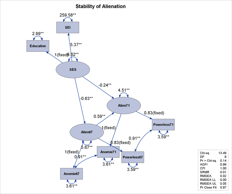
Output 29.17.8 shows the path diagram of the unstandardized solution. The path diagram indicates significant estimates by attaching asterisks
to the numerical values. Estimates that are flagged with one asterisk are significant at 0.05  -level. Estimates that are flagged with two asterisks are significant at 0.01 -level. The path diagram also shows a summary of fit statistics. For more information about specifying path diagram output,
see the section Path Diagrams: Layout Algorithms, Default Settings, and Customization.
-level. Estimates that are flagged with two asterisks are significant at 0.01 -level. The path diagram also shows a summary of fit statistics. For more information about specifying path diagram output,
see the section Path Diagrams: Layout Algorithms, Default Settings, and Customization.
Output 29.17.8: Path Diagram and Fit Summary
PROC CALIS can perform a detailed residual analysis. Large residuals might indicate misspecification of the model. In Output 29.17.9, raw residuals are reported and ranked.
Output 29.17.9: Raw Residuals and Ranking
| Raw Residual Matrix | |||||||
|---|---|---|---|---|---|---|---|
| Anomie67 | Powerless67 | Anomie71 | Powerless71 | Education | SEI | ||
| Anomie67 | Anomie (1967) | -0.06997 | 0.03642 | -0.01116 | -0.15200 | 0.32892 | 0.47786 |
| Powerless67 | Powerlessness (1967) | 0.03642 | 0.01261 | 0.15600 | 0.01135 | -0.41712 | -0.19108 |
| Anomie71 | Anomie (1971) | -0.01116 | 0.15600 | -0.08381 | -0.00854 | 0.22464 | 0.07976 |
| Powerless71 | Powerlessness (1971) | -0.15200 | 0.01135 | -0.00854 | 0.14067 | -0.23832 | -0.59248 |
| Education | Education | 0.32892 | -0.41712 | 0.22464 | -0.23832 | 0.00000 | 0.00000 |
| SEI | Occupational Status Index | 0.47786 | -0.19108 | 0.07976 | -0.59248 | 0.00000 | 0.00002 |
| Rank Order of the 10 Largest Raw Residuals | ||
|---|---|---|
| Var1 | Var2 | Residual |
| SEI | Powerless71 | -0.59248 |
| SEI | Anomie67 | 0.47786 |
| Education | Powerless67 | -0.41712 |
| Education | Anomie67 | 0.32892 |
| Education | Powerless71 | -0.23832 |
| Education | Anomie71 | 0.22464 |
| SEI | Powerless67 | -0.19108 |
| Anomie71 | Powerless67 | 0.15600 |
| Powerless71 | Anomie67 | -0.15200 |
| Powerless71 | Powerless71 | 0.14067 |
Because of the differential scaling of the variables, it is usually more useful to examine the standardized residuals instead. In Output 29.17.10, for example, the table for the 10 largest asymptotically standardized residuals is displayed.
Output 29.17.10: Asymptotically Standardized Residuals and Ranking
| Asymptotically Standardized Residual Matrix | |||||||
|---|---|---|---|---|---|---|---|
| Anomie67 | Powerless67 | Anomie71 | Powerless71 | Education | SEI | ||
| Anomie67 | Anomie (1967) | -0.30882 | 0.52686 | -0.05619 | -0.86507 | 2.55338 | 0.46484 |
| Powerless67 | Powerlessness (1967) | 0.52686 | 0.05464 | 0.87613 | 0.05735 | -2.76371 | -0.17015 |
| Anomie71 | Anomie (1971) | -0.05619 | 0.87613 | -0.35460 | -0.12169 | 1.69781 | 0.07009 |
| Powerless71 | Powerlessness (1971) | -0.86507 | 0.05735 | -0.12169 | 0.58521 | -1.55750 | -0.49608 |
| Education | Education | 2.55338 | -2.76371 | 1.69781 | -1.55750 | 0.00000 | 0.00000 |
| SEI | Occupational Status Index | 0.46484 | -0.17015 | 0.07009 | -0.49608 | 0.00000 | 0.00000 |
| Rank Order of the 10 Largest Asymptotically Standardized Residuals | ||
|---|---|---|
| Var1 | Var2 | Residual |
| Education | Powerless67 | -2.76371 |
| Education | Anomie67 | 2.55338 |
| Education | Anomie71 | 1.69781 |
| Education | Powerless71 | -1.55750 |
| Anomie71 | Powerless67 | 0.87613 |
| Powerless71 | Anomie67 | -0.86507 |
| Powerless71 | Powerless71 | 0.58521 |
| Powerless67 | Anomie67 | 0.52686 |
| SEI | Powerless71 | -0.49608 |
| SEI | Anomie67 | 0.46484 |
The model performs the poorest concerning the covariances of Education with all measures of Powerless and Anomie. This might suggest a misspecification of the functional relationships of Education with other variables in the model. However, because the model fit is quite good, such a possible misspecification should
not be a serious concern in the analysis.
The histogram of the asymptotically standardized residuals is displayed in Output 29.17.11, which also shows the normal and kernel approximations.
Output 29.17.11: Distribution of Asymptotically Standardized Residuals
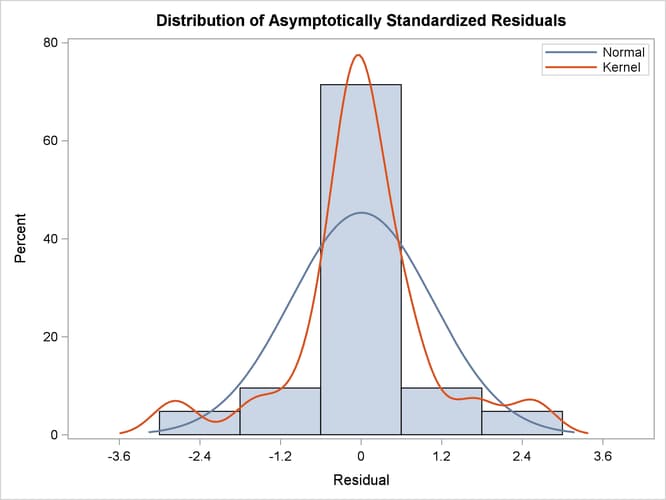
The residual distribution looks quite symmetrical. It shows a small to medium departure from the normal distribution, as evidenced by the discrepancies between the kernel and the normal distribution curves.
Output 29.17.12 shows the estimation results.
Output 29.17.12: Estimation Results
| PATH List | |||||||
|---|---|---|---|---|---|---|---|
| Path | Parameter | Estimate | Standard Error |
t Value | Pr > |t| | ||
| Anomie67 | <=== | Alien67 | 1.00000 | ||||
| Powerless67 | <=== | Alien67 | 0.83300 | ||||
| Anomie71 | <=== | Alien71 | 1.00000 | ||||
| Powerless71 | <=== | Alien71 | 0.83300 | ||||
| Education | <=== | SES | 1.00000 | ||||
| SEI | <=== | SES | lambda | 5.36883 | 0.43371 | 12.3788 | <.0001 |
| Alien67 | <=== | SES | gamma1 | -0.62994 | 0.05634 | -11.1809 | <.0001 |
| Alien71 | <=== | SES | gamma2 | -0.24086 | 0.05489 | -4.3884 | <.0001 |
| Alien71 | <=== | Alien67 | beta | 0.59312 | 0.04678 | 12.6788 | <.0001 |
| Variance Parameters | ||||||
|---|---|---|---|---|---|---|
| Variance Type |
Variable | Parameter | Estimate | Standard Error |
t Value | Pr > |t| |
| Error | Anomie67 | theta1 | 3.60796 | 0.20092 | 17.9572 | <.0001 |
| Powerless67 | theta2 | 3.59488 | 0.16448 | 21.8556 | <.0001 | |
| Anomie71 | theta1 | 3.60796 | 0.20092 | 17.9572 | <.0001 | |
| Powerless71 | theta2 | 3.59488 | 0.16448 | 21.8556 | <.0001 | |
| Education | theta3 | 2.99366 | 0.49861 | 6.0040 | <.0001 | |
| SEI | theta4 | 259.57639 | 18.31151 | 14.1756 | <.0001 | |
| Alien67 | psi1 | 5.67046 | 0.42301 | 13.4050 | <.0001 | |
| Alien71 | psi2 | 4.51479 | 0.33532 | 13.4639 | <.0001 | |
| Exogenous | SES | phi | 6.61634 | 0.63914 | 10.3519 | <.0001 |
The paths, variances and partial (or error) variances, and covariances and partial covariances are shown. When you have fixed
parameters such as the first five path coefficients in the output, the standard errors and t values are all blanks. For free or constrained estimates, standard errors and t values are computed. Researchers in structural equation modeling usually use the value 2 as an approximate critical value
for the observed t values. The reason is that the estimates are asymptotically normal, and so the two-sided critical point with  is 1.96, which is close to 2. Using this criterion, all estimates shown in Output 29.17.12 are significantly different from zero, supporting the presence of these parameters in the model.
Squared multiple correlations are shown in Output 29.17.13.
Output 29.17.13: Squared Multiple Correlations
| Squared Multiple Correlations | |||
|---|---|---|---|
| Variable | Error Variance | Total Variance | R-Square |
| Anomie67 | 3.60796 | 11.90397 | 0.6969 |
| Anomie71 | 3.60796 | 12.61581 | 0.7140 |
| Education | 2.99366 | 9.61000 | 0.6885 |
| Powerless67 | 3.59488 | 9.35139 | 0.6156 |
| Powerless71 | 3.59488 | 9.84533 | 0.6349 |
| SEI | 259.57639 | 450.28798 | 0.4235 |
| Alien67 | 5.67046 | 8.29601 | 0.3165 |
| Alien71 | 4.51479 | 9.00786 | 0.4988 |
For each endogenous variable in the model, the corresponding squared multiple correlation is computed by:
![\[ 1 - \frac{\mbox{error variance}}{\mbox{total variance}} \]](images/statug_calis0956.png)
In regression analysis, this is the percentage of explained variance of the endogenous variable by the predictors. However, this interpretation is complicated or even uninterpretable when your structural equation model has correlated errors or reciprocal casual relations. In these situations, it is not uncommon to see negative R-squares. Negative R-squares do not necessarily mean that your model is wrong or the model prediction is weak. Rather, the R-square interpretation is questionable in these situations.
When your variables are measured on different scales, comparison of path coefficients cannot be made directly. For example,
in Output 29.17.12, the path coefficient for path Education <=== SES is fixed at one, while the path coefficient for path SEI <=== SES is 5.369. It would be simple-minded to conclude that the effect of SES on SEI is greater than that SES on Education. Because SEI and Education are measured on different scales, direct comparison of the corresponding path coefficients is simply inappropriate.
In alleviating this problem, some might resort to the standardized solution for a better comparison. In a standardized solution, because the variances of manifest variables and systematic predictors are all standardized to ones, you hope the path coefficients are more comparable. In this example, PROC CALIS standardizes your results in Output 29.17.14.
Output 29.17.14: Standardized Results
| Standardized Results for PATH List | |||||||
|---|---|---|---|---|---|---|---|
| Path | Parameter | Estimate | Standard Error |
t Value | Pr > |t| | ||
| Anomie67 | <=== | Alien67 | 0.83481 | 0.01093 | 76.3531 | <.0001 | |
| Powerless67 | <=== | Alien67 | 0.78459 | 0.01163 | 67.4776 | <.0001 | |
| Anomie71 | <=== | Alien71 | 0.84499 | 0.01031 | 81.9796 | <.0001 | |
| Powerless71 | <=== | Alien71 | 0.79678 | 0.01107 | 71.9626 | <.0001 | |
| Education | <=== | SES | 0.82975 | 0.03172 | 26.1599 | <.0001 | |
| SEI | <=== | SES | lambda | 0.65079 | 0.03019 | 21.5533 | <.0001 |
| Alien67 | <=== | SES | gamma1 | -0.56257 | 0.03456 | -16.2796 | <.0001 |
| Alien71 | <=== | SES | gamma2 | -0.20642 | 0.04483 | -4.6043 | <.0001 |
| Alien71 | <=== | Alien67 | beta | 0.56920 | 0.04066 | 14.0000 | <.0001 |
| Standardized Results for Variance Parameters | ||||||
|---|---|---|---|---|---|---|
| Variance Type |
Variable | Parameter | Estimate | Standard Error |
t Value | Pr > |t| |
| Error | Anomie67 | theta1 | 0.30309 | 0.01825 | 16.6031 | <.0001 |
| Powerless67 | theta2 | 0.38442 | 0.01825 | 21.0695 | <.0001 | |
| Anomie71 | theta1 | 0.28599 | 0.01742 | 16.4178 | <.0001 | |
| Powerless71 | theta2 | 0.36514 | 0.01764 | 20.6942 | <.0001 | |
| Education | theta3 | 0.31152 | 0.05264 | 5.9182 | <.0001 | |
| SEI | theta4 | 0.57647 | 0.03930 | 14.6680 | <.0001 | |
| Alien67 | psi1 | 0.68352 | 0.03888 | 17.5797 | <.0001 | |
| Alien71 | psi2 | 0.50121 | 0.03321 | 15.0897 | <.0001 | |
| Exogenous | SES | phi | 1.00000 | |||
Now, the standardized path coefficient for path Education <=== SES is 0.830, while the standardized path coefficient for path SEI <=== SES is 0.651. So the standardized effect of SES on SEI is actually smaller than that of SES on Education.
Furthermore, in PROC CALIS the standardized estimates are computed with standard error estimates and t values so that you can make statistical inferences on the standardized estimates as well.
PROC CALIS might differ from other software in its standardization scheme. Unlike other software that might standardize the path coefficients that attach to the error terms (unsystematic sources), PROC CALIS keeps these path coefficients at ones (not shown in the output). Unlike other software that might also standardize the corresponding error variances to ones, the error variances in the standardized solution of PROC CALIS are rescaled so as to keep the mathematical consistency of the model.
Essentially, in PROC CALIS only variances of manifest and non-error-type latent variables are standardized to ones. The error
variances are rescaled, but not standardized. For example, in the standardized solution shown in Output 29.17.14, the error variances for all endogenous variables are not ones (see the middle portion of the output). Only the variance
for the latent variable SES is standardized to one. See the section Standardized Solutions for the logic of the standardization scheme adopted by PROC CALIS.
In appearance, the standardized solution is like a correlational analysis on the standardized manifest variables with standardized
exogenous latent factors. Unfortunately, this statement is over-simplified, if not totally inappropriate. In standardizing
a solution, the implicit equality constraints are likely destroyed. In this example, the unstandardized error variances for
Anomie67 and Anomie71 are both 3.608, represented by a common parameter theta1. However, after standardization, these error variances have different values at 0.303 and 0.286, respectively. In addition,
fixed parameter values are no longer fixed in a standardized solution (for example, the first five paths in the current example).
The issue of standardization is common to all other SEM software and beyond the current discussion. PROC CALIS provides the
standardized solution so that users can interpret the standardized estimates whenever they find them appropriate.