The CALIS Procedure

Example 29.8 Measurement Error Models

Subsections:

Measurement Error in x
Measurement Errors in x and y
Linear Regression Model as a Special Case of Structural Equation Model

In this example, you use PROC CALIS to fit some measurement error models. You use latent variables to define "true" scores variables that are measured without errors. You constrain parameters by using parameter names or fixed values in the PATH model specification.

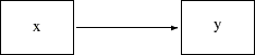
Consider a simple linear regression model with dependent variable y and predictor variable x. The path diagram for this simple linear regression model is depicted as follows:

Output 29.8.1:

Suppose you have the following SAS data set for the regression analysis of y on x:

data measures;
   input x y @@;
   datalines;
 7.91736    13.8673    6.10807    11.7966    6.94139    12.2174
 7.61290    12.9761    6.77190    11.6356    6.33328    11.7732
 7.60608    12.8040    6.65642    12.8866    6.26643    11.9382
 7.32266    13.2590    5.76977    10.7654    5.62881    11.5041
 7.57418    13.2502    7.17305    13.3416    8.23123    13.9876
 7.17199    13.1750    8.04604    14.5968    5.77692    11.5077
 5.72741    11.3299    6.66033    12.5159    7.14944    12.4988
 7.51832    12.3588    5.48877    11.2211    7.50323    13.3735
 7.15814    13.1556    7.35485    13.8457    8.91648    14.4929
 5.37445     9.6366    6.00419    11.7654    6.89546    13.1493
;

This data set contains 30 observations for the x and y variables. You can fit the simple linear regression model to the measures data by the PATH model specification of PROC CALIS, as shown in the following statements:

proc calis data=measures;
   path
      x ===> y;
run;

Output 29.8.2 shows that the regression coefficient estimate (denoted as _Parm1 in the PATH List) is 1.1511 (standard error = 0.1002).

Output 29.8.2: Estimates of the Linear Regression Model for the Measures Data

PATH List
Path			Parameter	Estimate	Standard Error	t Value	Pr > \|t\|
x	===>	y	_Parm1	1.15112	0.10016	11.4924	<.0001

Variance Parameters
Variance Type	Variable	Parameter	Estimate	Standard Error	t Value	Pr > \|t\|
Exogenous	x	_Add1	0.79962	0.20999	3.8079	0.0001
Error	y	_Add2	0.23265	0.06110	3.8079	0.0001

You can also do the simple linear regression by PROC REG by the following statement:

proc reg data=measures;
   model y = x;
run;

Output 29.8.3 shows that PROC REG essentially gives the same regression coefficient estimate with a similar standard error estimate. The discrepancy in the standard error estimates produced by the two procedures is due to the different variance divisors in computing standard errors in the two procedures. But the discrepancy is negligible when the sample size becomes large.

Output 29.8.3: PROC REG Estimates of the Linear Regression Model for the Measures Data

Parameter Estimates
Variable	DF	Parameter Estimate	Standard Error	t Value	Pr > \|t\|
Intercept	1	4.62455	0.70790	6.53	<.0001
x	1	1.15112	0.10194	11.29	<.0001

There are two main differences between PROC CALIS and PROC REG regarding the parameter estimation results. First, PROC CALIS does not give the estimate of the intercept because by default PROC CALIS analyzes only the covariance structures. Therefore, it does not estimate the intercept. To obtain the intercept estimate, you can add the MEANSTR option in the PROC CALIS statement, as is shown in Example 29.9. Second, in Output 29.8.2 of PROC CALIS, the variance estimate of x and the error variance estimate of y are shown. The corresponding results are not shown as parameter estimates in the PROC REG results. In PROC CALIS, these two variances are model parameters in covariance structure analysis. PROC CALIS adds these variances as default parameters. You can also represent these two variance parameters by double-headed arrows in the path diagram, as shown in the following:

Output 29.8.4:

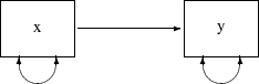
The two double headed-arrows attached to x and y represent the variances. Although it is not necessary to specify these default parameters, you can use the PVAR statement to specify them explicitly, as shown in the following statements:

proc calis data=measures meanstr;
   path
      x ===> y;
   pvar
      x y;
run;

In the PROC CALIS statement, you specify the MEANSTR option to request the analysis of mean structures together with covariance structures. Output 29.8.5 shows the estimation results.

Output 29.8.5: Estimates of the Measurement Error Model with Error in x

PATH List
Path			Parameter	Estimate	Standard Error	t Value	Pr > \|t\|
x	===>	y	_Parm1	1.15112	0.10016	11.4924	<.0001

Variance Parameters
Variance Type	Variable	Parameter	Estimate	Standard Error	t Value	Pr > \|t\|
Exogenous	x	_Parm2	0.79962	0.20999	3.8079	0.0001
Error	y	_Parm3	0.23265	0.06110	3.8079	0.0001

Means and Intercepts
Type	Variable	Parameter	Estimate	Standard Error	t Value	Pr > \|t\|
Intercept	y	_Add1	4.62455	0.69578	6.6466	<.0001
Mean	x	_Add2	6.88865	0.16605	41.4850	<.0001

The regression coefficient estimate and the variance estimates are the same as those in Output 29.8.2. However, in Output 29.8.5, there is an additional table for the mean and intercept estimates. The intercept estimate for y is 4.6246 (standard error=0.6958), which match closely to the results obtained from PROC REG, as shown in Output 29.8.3.

Measurement Error in x

PROC CALIS can also handle more complicated regression situations where the variables are measured with errors. This is beyond the application of PROC REG.

Suppose that the predictor variable x is measured with error and from prior studies you know that the size of the measurement error variance is about 0.019. You can use PROC CALIS to incorporate this information into the model. First, think of the measured variable x as composed of two components: one component is the "true" score measure Fx and the other is the measurement error e1. Both of these components are not observed (that is, latent) but they sum up to yield x. That is,

$\mbox{x} = \mbox{Fx} + \mbox{e1}$

Because x is contaminated with measurement error, what you are interested in knowing is the regression effect of the true score Fx on x. The following path diagram represents this regression scenario:

Output 29.8.6:

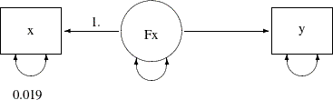
In path diagrams, latent variables are usually represented by circles or ovals, while observed variables are represented by rectangles. In the current path diagram, Fx is a latent variable and is represented by a circle. The other two variables are observed variables and are represented by rectangles. There are five arrows in the path diagram. Two of them are single-headed arrows that represent functional relationships, while the other three are double-headed arrows that represent variances or error variances. Two paths are labeled with fixed values. The path effect from Fx to x is fixed at 1, as assumed in the measurement error model. The error variance for measuring x is fixed at 0.019 due to the prior knowledge about the measurement error variance. The remaining three arrows represent free parameters in the model: the regression coefficient of y on Fx, the variance of Fx, and the error variance of y. The following statements specify the model for this path diagram:

proc calis data=measures;
   path
      x  <=== Fx   = 1.,
      Fx ===> y;
   pvar
      x  = 0.019,
      Fx, y;
run;

You specify all the single-headed paths in the PATH statement and all the double-headed arrows in the PVAR statement. For paths with fixed values, you put the equality at the back of the specifications to tell PROC CALIS about the fixed values. For example, the path coefficient in the path x <=== Fx is fixed at 1 and the error variance for x is fixed at 0.019. All other specifications represent unnamed free parameters in the model.

Output 29.8.7 shows the estimation results. The effect of Fx on y is 1.1791 (standard error=0.1029). This effect is slightly greater than the corresponding effect (1.1511) of x on y in the preceding model where the measurement error of x has not been taken into account, as shown in Output 29.8.5.

Output 29.8.7: Estimates of the Measurement Error Model with Error in x

PATH List
Path			Parameter	Estimate	Standard Error	t Value	Pr > \|t\|
x	<===	Fx		1.00000
Fx	===>	y	_Parm1	1.17914	0.10288	11.4615	<.0001

Variance Parameters
Variance Type	Variable	Parameter	Estimate	Standard Error	t Value	Pr > \|t\|
Error	x		0.01900
Exogenous	Fx	_Parm2	0.78062	0.20999	3.7174	0.0002
Error	y	_Parm3	0.20686	0.06126	3.3767	0.0007

Measurement Errors in x and y

Measurement error can occur in the y variable too. Suppose that both x and y are measured with errors. From prior studies, the measurement error variance of x is known to be 0.019 (as in the preceding modeling scenario) and the measurement error variance of y is known to be 0.022. The following path diagram represents the current modeling scenario:

Output 29.8.8:

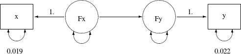
In the current path diagram the true score variable Fy and its measurement indicator y have the same kind of relationship as the relationship between the true score variable Fx and its measurement indicator x in the previous description. The error variance for measuring y is treated as a known constant 0.022. You can transcribe this path diagram easily to the following PROC CALIS specification:

proc calis data=measures;
   path
      x  <=== Fx  = 1.,
      Fx ===> Fy   ,
      Fy ===> y   = 1.;
   pvar
      x  = 0.019,
      y  = 0.022,
      Fx Fy;
run;

Again, you specify all the single-headed paths in the PATH statement and the double-headed paths in the PVAR statement. You provide the fixed parameter values by appending the required equalities after the individual specifications.

Output 29.8.9 shows the estimation results of the model with measurement errors in both x and y. The effect of Fx on Fy is 1.1791 (standard error=0.1029). This is essentially the same effect of Fx on y as in the preceding measurement model in which no measurement error in y is assumed.

Output 29.8.9: Estimates of the Measurement Error Model with Errors in x and y

PATH List
Path			Parameter	Estimate	Standard Error	t Value	Pr > \|t\|
x	<===	Fx		1.00000
Fx	===>	Fy	_Parm1	1.17914	0.10288	11.4615	<.0001
Fy	===>	y		1.00000

Variance Parameters
Variance Type	Variable	Parameter	Estimate	Standard Error	t Value	Pr > \|t\|
Error	x		0.01900
	y		0.02200
Exogenous	Fx	_Parm2	0.78062	0.20999	3.7174	0.0002
Error	Fy	_Parm3	0.18486	0.06126	3.0176	0.0025

The estimated error variance for Fy in the current model is 0.1849 and the measurement error variance of y is fixed at 0.022, as shown in the last table of Output 29.8.9. The sum is 0.2069, which is the same amount of error variance for y in the preceding model with measurement error assumed only in x. Hence, the assumption of the measurement error in y does not change the structural effect of Fx on y (same amount of effect Fx on Fy, which is 1.1791). It only changes the variance components of y. In the preceding model with measurement error assumed only in x, the total error variance in y is 0.2069. In the current model, this total error variance is partitioned into the measurement error variance (which is fixed at 0.022) and the error variance in the regression on Fx (which is estimated at 0.1849).

Linear Regression Model as a Special Case of Structural Equation Model

By using the current measurement error model as an illustration, it is easy to see that the structural equation model is a more general model that includes the linear regression model as a special case. If you restrict the measurement error variances in x and y to zero, the measurement error model (which represents the structural equation model in this example) reduces to the linear regression model. That is, the path diagram becomes:

Output 29.8.10:

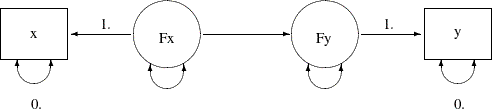
You can then specify the PATH model by the following statements:

proc calis data=measures;
   path
      x  <=== Fx  = 1.,
      Fx ===> Fy   ,
      Fy ===> y   = 1.;
   pvar
      x  = 0.,
      y  = 0.,
      Fx Fy;
run;

Output 29.8.11 shows the estimation results of this measurement error model with zero measurement errors. The estimate of the regression coefficient is 1.1511, which is essentially the same result as in Output 29.8.3 by using PROC REG.

Output 29.8.11: Estimates of the Measurement Error Model with Zero Measurement Errors

PATH List
Path			Parameter	Estimate	Standard Error	t Value	Pr > \|t\|
x	<===	Fx		1.00000
Fx	===>	Fy	_Parm1	1.15112	0.10016	11.4924	<.0001
Fy	===>	y		1.00000

Variance Parameters
Variance Type	Variable	Parameter	Estimate	Standard Error	t Value	Pr > \|t\|
Error	x		0
	y		0
Exogenous	Fx	_Parm2	0.79962	0.20999	3.8079	0.0001
Error	Fy	_Parm3	0.23265	0.06110	3.8079	0.0001

This example shows that you can apply PROC CALIS to fit measurement error models. You treat true scores variables as latent variables in the structural equation model. The linear regression model is a special case of the structural equation model (or measurement error model) where measurement error variances are assumed to be zero. Structural equation modeling by PROC CALIS is not limited to this simple modeling scenario. PROC CALIS can treat more complicated measurement error models. In Example 29.9 and Example 29.10, you fit measurement error models with parameter constraints and with more than one predictor. You can also fit measurement error models with correlated errors.