The CALIS Procedure

Loehlin (1987) analyzes the following path model for the data:

Output 29.24.1: Path Diagram for Career Aspiration: Model 1

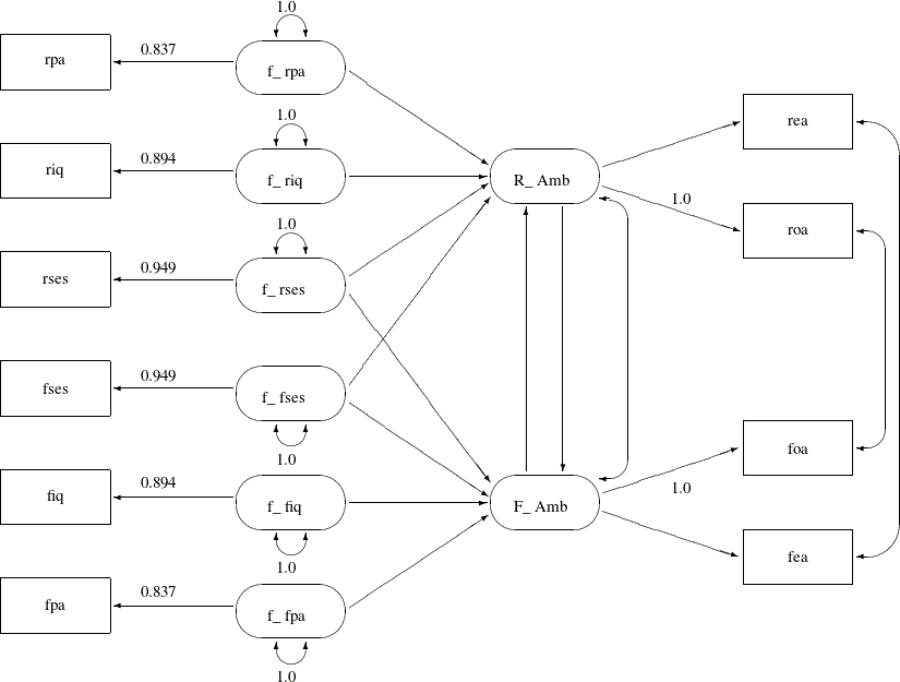
In Output 29.24.1, the observed variables rpa, riq, rses, fses, fiq, and fpa are measured with errors. Their true scores counterparts f_rpa, f_riq, f_rses, f_fses, f_fiq, and f_fpa are latent variables in the model. Path coefficients from these latent variables to the observed variables are fixed coefficients, indicating the square roots of the theoretical reliabilities in the model. These latent variables, rather than the observed counterparts, serve as predictors of the ambition factors R_Amb and F_Amb. The error terms for these two latent factors are correlated, as indicated by a double-headed path (arrow) that connects the two factors. Correlated errors for the occupational aspiration variables (roa and foa) and the educational aspiration variables (rea and fea) are also shown in Output 29.24.1. These correlated errors are also represented by two double-headed paths (arrows) in the path diagram.

Notice that the covariances among the six exogenous latent variables (f_rpa, f_riq, f_rses, f_fses, f_fiq, and f_fpa) are not represented in the path diagram for two reasons. First, there are 15 of these covariances and hence you need 15 double-headed arrows to represent them in the path diagram. Apparently, because of the space limitations, it would be difficult to put all these double-headed arrows in the path diagram without cluttering it. Second, covariances among exogenous latent variables are free parameters by default in PROC CALIS, and therefore omitting these double-headed arrows in the path diagram is compatible with the default model specification in PROC CALIS. Similarly, double-headed arrows for the error variances of the endogenous variables (rpa, riq, rses, fses, fiq, fpa, R_Amb, and F_Amb) in the path diagram are omitted because they are unconstrained free parameters and are set automatically by default in PROC CALIS .

The model represented by the path diagram in Output 29.24.1 is considered to be the full model for the data, in the sense that it has the largest number of parameters among the competing models considered this example. The same model is analyzed in the section A Combined Measurement-Structural Model in Chapter 17: Introduction to Structural Equation Modeling with Latent Variables, with the following specification:

proc calis data=aspire nobs=329;
   path
      /* measurement model for intelligence and environment */
      rpa     <===  f_rpa    = 0.837,
      riq     <===  f_riq    = 0.894,
      rses    <===  f_rses   = 0.949,
      fses    <===  f_fses   = 0.949,
      fiq     <===  f_fiq    = 0.894,
      fpa     <===  f_fpa    = 0.837,

      /* structural model of influences: 5 equality constraints */
      f_rpa   ===>  R_Amb ,
      f_riq   ===>  R_Amb ,
      f_rses  ===>  R_Amb ,
      f_fses  ===>  R_Amb ,
      f_rses  ===>  F_Amb ,
      f_fses  ===>  F_Amb ,
      f_fiq   ===>  F_Amb ,
      f_fpa   ===>  F_Amb ,
      F_Amb   ===>  R_Amb ,
      R_Amb   ===>  F_Amb ,

      /* measurement model for aspiration: 1 equality constraint */
      R_Amb   ===>  rea  ,
      R_Amb   ===>  roa      = 1.,
      F_Amb   ===>  foa      = 1.,
      F_Amb   ===>  fea  ;
   pvar
      f_rpa f_riq f_rses f_fpa f_fiq f_fses = 6 * 1.0;
   pcov
      R_Amb F_Amb            ,
      rea  fea               ,
      roa  foa               ;
run;

The PATH model specification represents each arrow (single-headed and double-headed) in the path diagram. You transcribe each arrow in Output 29.24.1 into an entry in the PATH model. The PATH statement specifies all the single-headed arrows in the path diagram. The PVAR statement specifies all the double-headed arrows that point to individual variables (that is, the fixed error variances of the exogenous latent variables) in the path diagram. The PCOV statement specifies all the double-headed arrows that connect paired variables (that is, the error covariances) in the path diagram.

Output 29.24.2 shows the fit summary of Model 1.

Since the p-value for the chi-square test is 0.5266, this model clearly cannot be rejected. Both standardized RMR and RMSEA are very small. All these point to an excellent model fit. Three information-theoretic fit indices are also shown: Akaike’s information criterion (AIC), Bozdogan’s CAIC, and Schwarz’s Bayesian Criterion (SBC). These indices are useful when you need to compare competing models for the data.

You now consider a much more restrictive model with equality constraints in the model. The path diagram for this constrained model is shown in Output 29.24.3.

Output 29.24.3: Path Diagram for Career Aspiration: Model 2

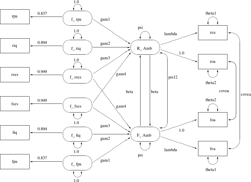
The main idea about setting the equality constraints in this model is that there is some symmetry in the model components that correspond to the respondent and his friend. In particular, the corresponding coefficients or parameters should be equal. For example, the path f_rpa===>R_Amb for the respondent has the same effect as that of f_fpa===>F_Amb. In the path diagram, they are both labeled by the same parameter gam1. Generalizing the same idea to other pairs of paths, Output 29.24.3 shows nine pairs of these equality constraints, which are all represented by the same parameter names for distinct (single-headed or double-headed) paths.

However, because of the space limitation, there are six more equality constraints that are not shown in the path diagram. These six constraints concern the covariance structures of the exogenous latent factors f_rpa, f_riq, f_rses, f_fses, f_fiq, and f_fpa. The first three factors are for the respondent, and the last three are for his friend. Using the same symmetry argument, the covariance structures imposed on these exogenous latent factors are shown in the following:

         f_rpa  f_riq  f_rses   f_fpa f_fiq f_fses
f_rpa      1.
f_riq      c1     1.
f_rses     c2     c3     1.

f_fpa      c4     c5     c6       1.
f_fiq      c5     c7     c8       c1    1.
f_fses     c6     c8     c9       c2    c3    1.

In this pattern of covariance structures, the covariance matrix (upper left portion) for the latent factors of the respondent is the same as that (lower right portion) for the latent factors of his friend. The cross-covariances among the factors between the friends (lower left portion) also display a symmetry pattern. There are six pairs of equality constraints in the covariance structures. Imposing these six pairs of equality constraints and the nine pairs of equality constraints in the path diagram lead to Model 2 of Loehlin (1987).

You can specify the current constrained model by the following PATH modeling language of PROC CALIS:

proc calis data=aspire nobs=329 outmodel=model2;
   path
      /* measurement model for intelligence and environment */
      rpa     <===  f_rpa    = 0.837,
      riq     <===  f_riq    = 0.894,
      rses    <===  f_rses   = 0.949,
      fses    <===  f_fses   = 0.949,
      fiq     <===  f_fiq    = 0.894,
      fpa     <===  f_fpa    = 0.837,

      /* structural model of influences: 5 equality constraints */
      f_rpa   ===>  R_Amb    = gam1,
      f_riq   ===>  R_Amb    = gam2,
      f_rses  ===>  R_Amb    = gam3,
      f_fses  ===>  R_Amb    = gam4,
      f_rses  ===>  F_Amb    = gam4,
      f_fses  ===>  F_Amb    = gam3,
      f_fiq   ===>  F_Amb    = gam2,
      f_fpa   ===>  F_Amb    = gam1,
      F_Amb   ===>  R_Amb    = beta,
      R_Amb   ===>  F_Amb    = beta,

      /* measurement model for aspiration: 1 equality constraint */
      R_Amb   ===>  rea      = lambda,
      R_Amb   ===>  roa      = 1.,
      F_Amb   ===>  foa      = 1.,
      F_Amb   ===>  fea      = lambda;
   pvar
      f_rpa f_riq f_rses f_fpa f_fiq f_fses = 6 * 1.0,
      R_Amb F_Amb             = 2 * psi,        /* 1 ec */
      rea fea                 = 2 * theta1,     /* 1 ec */
      roa foa                 = 2 * theta2;     /* 1 ec */
   pcov
      R_Amb F_Amb             = psi12,
      rea  fea                = covea,
      roa  foa                = covoa,
      f_rpa f_riq f_rses      = cov1-cov3,       /* 3 ec */
      f_fpa f_fiq f_fses      = cov1-cov3,
      f_rpa f_riq f_rses * f_fpa f_fiq f_fses =  /* 3 ec */
          cov4 cov5 cov6  cov5 cov7 cov8  cov6 cov8 cov9;
run;

In the current PATH model specification, you specify the same set of paths as in Model 1. In addition, to set the required constraints in this path model, you use parameter names to label the related paths, variances, or covariances. Same parameter names mean equality constraints. The 15 equality constraints are labeled with comments in the specification. In the PROC CALIS statement, you use the OUTMODEL= option to output the model estimation results into the output data set model2, which is used for subsequent hypotheses tests.

Output 29.24.4 shows the fit summary of Model 2.

The test of Model 2 against Model 1 (Loehlin 1987) yields a chi-square of 19.0697 – 12.0132 = 7.0565 with 15 degrees of freedom, which is clearly not significant. This indicates that the restricted Model 2 fits at least as well as Model 1. Schwarz’s Bayesian criterion (SBC) is also much lower for Model 2 (175.5623) than for Model 1 (255.4476). Hence, Model 2 seems preferable on both substantive and statistical grounds.

A question of substantive interest is whether the friend’s socioeconomic status (SES) has a significant direct influence on a boy’s ambition. This can be addressed by omitting the paths from f_fses to R_Amb and from f_rses to F_Amb designated by the parameter name gam4, yielding Model 3 of Loehlin (1987). The corresponding path diagram is shown in Output 29.24.5.

Output 29.24.5: Path Diagram for Career Aspiration: Model 3

In Output 29.24.5, you drop the paths f_rses===>F_Amb and f_fses===>R_Amb from the previous model. Using the path diagram in Output 29.24.5, you can specify the current model the same way you do for Model 2. However, because you have the estimation results from Model 2 in the SAS data set model2, you can modify this SAS data set to reflect the current model specification and then input the modified SAS data set as an INMODEL= file for PROC CALIS to analyze.

First, you create a new SAS data set model3 by the following DATA step:

data model3(type=calismdl);
   set model2;
   if _name_='gam4' then
      do;
         _name_=' ';
         _estim_=0;
      end;
run;

Essentially, by blanking out the parameter name for the target paths, you are stating that these paths are no longer associated with the free parameter gam4 in the new model. Instead, you put a fixed zero to these paths. This way you eliminate the paths f_rses===>F_Amb and f_fses===>R_Amb for Model 3, of which the model specification is now saved in the model3 data set.

Next, you input model3 as the INMODEL= data set for PROC CALIS to analyze, as shown in the following statements:

proc calis data=aspire nobs=329 inmodel=model3;
run;

PROC CALIS can now use the previous estimation results for fitting the required model. Output 29.24.6 shows the fit summary of Model 3.

The chi-square value for testing Model 3 versus Model 2 is 23.0365 – 19.0697 = 3.9668 with one degree of freedom and a p-value of 0.0464. The chi-square test shows a marginal significance, which means that the paths might be needed in the model. However, the SBC (173.7340) indicates that Model 3 is slightly preferable to Model 2, which has an SBC value of 175.5632.

Another important question is whether the reciprocal influences between the respondent’s and friend’s ambitions are needed in the model. To test whether these paths are zero, you can set the parameter beta for the paths linking R_Amb and F_Amb to zero to obtain Model 4 of Loehlin (1987).

Similar to Model 3, you can modify the model2 data set to form the new model data set model4 for PROC CALIS to analyze, as shown in the following statements:

data model4(type=calismdl);
   set model2;
   if _name_='beta' then
      do;
         _name_=' ';
         _estim_=0;
      end;
run;

proc calis data=aspire nobs=329 inmodel=model4;
run;

Output 29.24.7 shows the fit summary of Model 4.

The chi-square value for testing Model 4 versus Model 2 is 20.9981 – 19.0697 = 1.9284 with one degree of freedom and a p-value of 0.1649. Hence, there is little evidence of reciprocal influence.

Model 2 of Loehlin (1987) has the direct paths connecting the latent ambition factors R_Amb and F_Amb and a covariance between the disturbance or error terms (that is, a double-headed arrow connecting the two factors in the path diagram shown in Output 29.24.3). The presence of this disturbance correlation serves as a "wastebasket" that enables other omitted variables to have joint influences on the respondent’s and his friend’s ambition factors. To test the hypothesis that this disturbance correlation is zero, you use the following statements to set the parameter psi12 to zero in the model5 data set and fit the new model by PROC CALIS:

data model5(type=calismdl);
   set model2;
   if _name_='psi12' then
      do;
         _name_=' ';
         _estim_=0;
      end;
run;

proc calis data=aspire nobs=329 inmodel=model5;
run;

Output 29.24.8 displays the fit summary of Model 5.

The chi-square value for testing Model 5 versus Model 2 is 19.0745 – 19.0697 = 0.0048 with one degree of freedom. This test statistic is insignificant. Therefore, omitting the covariance between the disturbance terms causes hardly any deterioration in the fit of the model.

The test in Model 4 fails to provide evidence of a direct reciprocal influence between the respondent’s and friend’s ambitions, and the test in Model 5 fails to provide evidence of a covariance or correlation between the disturbance terms for the ambition factors. Because you consider these two tests separately, you cannot establish evidence to eliminate the reciprocal influence and the disturbance correlation jointly. Instead, to make such a joint inference, it is important to test both hypotheses together by setting both beta and psi12 to zero as in Model 7 of Loehlin (1987). The following statements show how you can do that by modifying the model2 data set to form a new INMODEL= data set model7 for PROC CALIS to analyze:

data model7(type=calismdl);
   set model2;
   if _name_='psi12'|_name_='beta' then
      do;
         _name_=' ';
         _estim_=0;
      end;
run;

proc calis data=aspire nobs=329 inmodel=model7;
run;

Output 29.24.9 shows the fit summary of Model 7.

When Model 7 is tested against Models 2, 4, and 5, the p-values are respectively 0.0433, 0.0370, and 0.0123, indicating that the combined effect of the reciprocal influence and the covariance of the disturbance terms is statistically significant. Thus, the hypothesis tests indicate that it is acceptable to omit either the reciprocal influences or the covariance of the disturbances, but not both.

It is also of interest to test the covariances (covea and covoa) between the error terms for educational aspiration (that is, between rea and fea) and occupational aspiration (that is, between roa and foa), because these terms are omitted from Jöreskog and Sörbom (1988) models. Constraining covea and covoa to zero produces Model 6 of Loehlin (1987). You can use the following statements to fit this model:

data model6(type=calismdl);
   set model2;
   if _name_='covea'|_name_='covoa' then
      do;
         _name_=' ';
         _estim_=0;
      end;
run;

proc calis data=aspire nobs=329 inmodel=model6;
run;

Output 29.24.10 shows the fit summary of Model 6.

The chi-square value for testing Model 6 versus Model 2 is 33.4476 – 19.0697 = 14.3779 with two degrees of freedom and a p-value of 0.0008, indicating that there is considerable evidence of correlation between the error terms.

The following table summarizes the results from the seven models described in Loehlin (1987).

For comparing models, you can use a DATA step to compute the differences of the chi-square statistics and p-values, as shown in the following statements:

data _null_;
   array achisq[7] _temporary_
      (12.0132 19.0697 23.0365 20.9981 19.0745 33.4475 25.3466);
   array adf[7] _temporary_
      (13 28 29 29 29 30 30);
   retain indent 16;
   file print;
   input ho ha @@;
   chisq = achisq[ho] - achisq[ha];
   df = adf[ho] - adf[ha];
   p = 1 - probchi( chisq, df);
   if _n_ = 1 then put
      / +indent 'model comparison   chi**2   df  p-value'
      / +indent '---------------------------------------';
   put +indent +3 ho ' versus ' ha @18 +indent chisq 8.4 df 5. p 9.4;
   datalines;
2 1    3 2    4 2    5 2    7 2    7 4    7 5    6 2
;

The DATA step displays the table in Output 29.24.11.

                model comparison   chi**2   df  p-value                         
                ---------------------------------------                         
                   2  versus 1     7.0565   15   0.9561                         
                   3  versus 2     3.9668    1   0.0464                         
                   4  versus 2     1.9284    1   0.1649                         
                   5  versus 2     0.0048    1   0.9448                         
                   7  versus 2     6.2769    2   0.0433                         
                   7  versus 4     4.3485    1   0.0370                         
                   7  versus 5     6.2721    1   0.0123                         
                   6  versus 2    14.3778    2   0.0008                         

Although none of the seven models can be rejected when tested against the alternative of an unrestricted covariance matrix, the model comparisons make it clear that there are important differences among the models. Schwarz’s Bayesian criterion indicates Model 5 as the model of choice. The constraints added to Model 5 in Model 7 can be rejected (p = 0.0123), while Model 5 cannot be rejected when tested against the less constrained Model 2 (p = 0.9448). Hence, among the small number of models considered, Model 5 has strong statistical support. However, as Loehlin (1987, p.106) points out, many other models for these data could be constructed. Further analysis should consider, in addition to simple modifications of the models, the possibility that more than one friend could influence a boy’s aspirations, and that a boy’s ambition might have some effect on his choice of friends. Pursuing such theories would be statistically challenging.