The CALIS Procedure
-
Overview

-
Getting Started
-
SyntaxClasses of Statements in PROC CALISSingle-Group Analysis SyntaxMultiple-Group Multiple-Model Analysis SyntaxPROC CALIS StatementBOUNDS StatementBY StatementCOSAN StatementCOV StatementDETERM StatementEFFPART StatementFACTOR StatementFITINDEX StatementFREQ StatementGROUP StatementLINCON StatementLINEQS StatementLISMOD StatementLMTESTS StatementMATRIX StatementMEAN StatementMODEL StatementMSTRUCT StatementNLINCON StatementNLOPTIONS StatementOUTFILES StatementPARAMETERS StatementPARTIAL StatementPATH StatementPATHDIAGRAM StatementPCOV StatementPVAR StatementRAM StatementREFMODEL StatementRENAMEPARM StatementSAS Programming StatementsSIMTESTS StatementSTD StatementSTRUCTEQ StatementTESTFUNC StatementVAR StatementVARIANCE StatementVARNAMES StatementWEIGHT Statement
-
DetailsInput Data SetsOutput Data SetsDefault Analysis Type and Default ParameterizationThe COSAN ModelThe FACTOR ModelThe LINEQS ModelThe LISMOD Model and SubmodelsThe MSTRUCT ModelThe PATH ModelThe RAM ModelNaming Variables and ParametersSetting Constraints on ParametersAutomatic Variable SelectionPath Diagrams: Layout Algorithms, Default Settings, and CustomizationEstimation CriteriaRelationships among Estimation CriteriaGradient, Hessian, Information Matrix, and Approximate Standard ErrorsCounting the Degrees of FreedomAssessment of FitCase-Level Residuals, Outliers, Leverage Observations, and Residual DiagnosticsLatent Variable ScoresTotal, Direct, and Indirect EffectsStandardized SolutionsModification IndicesMissing Values and the Analysis of Missing PatternsMeasures of Multivariate KurtosisInitial EstimatesUse of Optimization TechniquesComputational ProblemsDisplayed OutputODS Table NamesODS Graphics
-
ExamplesEstimating Covariances and CorrelationsEstimating Covariances and Means SimultaneouslyTesting Uncorrelatedness of VariablesTesting Covariance PatternsTesting Some Standard Covariance Pattern HypothesesLinear Regression ModelMultivariate Regression ModelsMeasurement Error ModelsTesting Specific Measurement Error ModelsMeasurement Error Models with Multiple PredictorsMeasurement Error Models Specified As Linear EquationsConfirmatory Factor ModelsConfirmatory Factor Models: Some VariationsResidual Diagnostics and Robust EstimationThe Full Information Maximum Likelihood MethodComparing the ML and FIML EstimationPath Analysis: Stability of AlienationSimultaneous Equations with Mean Structures and Reciprocal PathsFitting Direct Covariance StructuresConfirmatory Factor Analysis: Cognitive AbilitiesTesting Equality of Two Covariance Matrices Using a Multiple-Group AnalysisTesting Equality of Covariance and Mean Matrices between Independent GroupsIllustrating Various General Modeling LanguagesTesting Competing Path Models for the Career Aspiration DataFitting a Latent Growth Curve ModelHigher-Order and Hierarchical Factor ModelsLinear Relations among Factor LoadingsMultiple-Group Model for Purchasing BehaviorFitting the RAM and EQS Models by the COSAN Modeling LanguageSecond-Order Confirmatory Factor AnalysisLinear Relations among Factor Loadings: COSAN Model SpecificationOrdinal Relations among Factor LoadingsLongitudinal Factor Analysis
- References
The LISMOD Model and Submodels
As a statistical model, the LISMOD modeling language is derived from the LISREL model proposed by Jöreskog and others (see Keesling 1972; Wiley 1973; Jöreskog 1973). But as a computer language, the LISMOD modeling language is quite different from the LISREL program. To maintain the consistence of specification syntax within the CALIS procedure, the LISMOD modeling language departs from the original LISREL programming language. In addition, to make the programming a little easier, some terminological changes from LISREL are made in LISMOD.
For brevity, models specified by the LISMOD modeling language are called LISMOD models, although you can also specify these LISMOD models by other general modeling languages that are supported in PROC CALIS.
The following descriptions of LISMOD models are basically the same as those of the original LISREL models. The main modifications are the names for the model matrices.
The LISMOD model is described by three component models. The first one is the structural equation model that describes the relationships among latent constructs or factors. The other two are measurement models that relate latent factors to manifest variables.
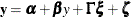
Structural Equation Model
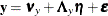
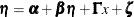
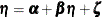
The structural equation model for latent factors is
![\[ \bm {\eta } = \balpha + \bbeta \bm {\eta } + \bGamma \bxi + \bzeta \]](images/statug_calis0343.png)
where:  is a random vector of
  endogenous latent factors
  is a random vector of
  exogenous latent factors
  is a random vector of errors
  is a vector of intercepts
  is a matrix of regression coefficients of variables on other variables
  is a matrix of regression coefficients of on
There are some assumptions in the structural equation model. To prevent a random variable in from regressing directly on itself, the diagonal elements of are assumed to be zeros. Also,  is assumed to be nonsingular, and is uncorrelated with .
The covariance matrix of is denoted by  and its expected value is a null vector. The covariance matrix of is denoted by
  and its expected value is denoted by
  .
.
Because variables in the structural equation model are not observed, to analyze the model these latent variables must somehow relate to the manifest variables. The measurement models, which are discussed in the subsequent sections, provide such relations.
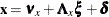
Measurement Model for 
![\[ \mb{y} = \bnu _ y + \bLambda _ y\bm {\eta } + \bepsilon \]](images/statug_calis0352.png)
where:  is a random vector of
  manifest variables
  is a random vector of errors for
  is a vector of intercepts for
  is a matrix of regression coefficients of on
It is assumed that is uncorrelated with either or . The covariance matrix of is denoted by  and its expected value is the null vector.
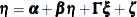
Measurement Model for 
![\[ \mb{x} = \bnu _ x + \bLambda _ x\bxi + \bdelta \]](images/statug_calis0358.png)
where:  is a random vector of
  manifest variables
  is a random vector of errors for
  is a vector of intercepts for
  is a matrix of regression coefficients of on
It is assumed that is uncorrelated with , , or . The covariance matrix of is denoted by  and its expected value is a null vector.
Covariance and Mean Structures
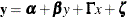
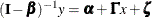
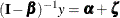
Under the structural and measurement equations and the model assumptions, the covariance structures of the manifest variables
 are expressed as
![\[ \bSigma = \left( \begin{matrix} \bLambda _ y (I - \bbeta )^{-1} (\bGamma \bPhi \bGamma ^\prime + \bPsi )(I - \bbeta ^\prime )^{-1} \bLambda _ y^\prime + \bTheta _ y & \bLambda _ y (I - \bbeta )^{-1}\bGamma \bPhi \bLambda _ x^\prime \\ \bLambda _ x\bPhi \bGamma ^\prime (I - \bbeta ^\prime )^{-1}\bLambda _ y^\prime & \bLambda _ x\bPhi \bLambda _ x^\prime + \bTheta _ x \\ \end{matrix} \right) \]](images/statug_calis0364.png)
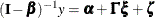
The mean structures of the manifest variables are expressed as
![\[ \bmu = \left( \begin{matrix} \bnu _ y + \bLambda _ y (I - \bbeta )^{-1} (\balpha + \bGamma \bkappa ) \\ \bnu _ x + \bLambda _ x \bkappa \\ \end{matrix} \right) \]](images/statug_calis0365.png)
Model Matrices in the LISMOD Model
The parameters of the LISMOD model are elements in the model matrices, which are summarized as follows.
|
Matrix |
Name |
Description |
Dimensions |
Row Variables |
Column Variables |
|---|---|---|---|---|---|
|
|
_ALPHA_ |
Intercepts for |
|
|
N/A |
|
|
_BETA_ |
Effects of |
|
|
|
|
|
_GAMMA_ |
Effects of |
|
|
|
|
|
_PSI_ |
Error covariance matrix for |
|
|
|
|
|
_PHI_ |
Covariance matrix for |
|
|
|
|
|
_KAPPA_ |
Mean vector for |
|
|
N/A |
|
|
_NUY_ |
Intercepts for |
|
|
N/A |
|
|
_LAMBDAY_ |
Effects of |
|
|
|
|
|
_THETAY_ |
Error covariance matrix for |
|
|
|
|
|
_NUX_ |
Intercepts for |
|
|
N/A |
|
|
_LAMBDAX_ |
Effects of |
|
|
|
|
|
_THETAX_ |
Error covariance matrix for |
|
|
|


There are twelve model matrices in the LISMOD model. Not all of them are used in all situations. See the section LISMOD Submodels for details. In the preceding table, each model matrix is given a name in the column Name, followed by a brief description of the parameters in the matrix, the dimensions, and the row and column variables being
referred to. In the second column of the table, the LISMOD matrix names are used in the MATRIX
statements when specifying the LISMOD model. In the last two columns of the table, following the row or column variables
is the variable list (for example, ETAVAR=, YVAR=, and so on) in parentheses. These lists are used in the LISMOD statement
for defining variables.
Specification of the LISMOD Model
The LISMOD specification consists of two tasks. The first task is to define the variables in the model. The second task is to specify the parameters in the LISMOD model matrices.
Specifying Variables
The first task is accomplished in the LISMOD statement
. In the LISMOD
statement, you define the lists of variables of interest: YVAR=, XVAR=, ETAVAR=, and XIVAR= lists, respectively for the -variables, -variables, -variables, and the -variables. While you provide the names of variables in these lists, you also define implicitly the numbers of four types
of variables: , , , and  . The variables in the YVAR= and XVAR= lists are manifest variables and therefore must be present in the analyzed data set.
The variables in the ETAVAR= and XIVAR= lists are latent factors, the names of which are assigned by the researcher to represent
their roles in the substantive theory. After these lists are defined, the dimensions of the model matrices are also defined
by the number of variables on various lists. In addition, the variable orders in the lists are referred to by the row and
column variables of the model matrices.
. The variables in the YVAR= and XVAR= lists are manifest variables and therefore must be present in the analyzed data set.
The variables in the ETAVAR= and XIVAR= lists are latent factors, the names of which are assigned by the researcher to represent
their roles in the substantive theory. After these lists are defined, the dimensions of the model matrices are also defined
by the number of variables on various lists. In addition, the variable orders in the lists are referred to by the row and
column variables of the model matrices.
Unlike the LINEQS model, in the LISMOD model you do not need to use the 'F' or 'f' prefix to denote factors in the ETAVAR= or XIVAR= list. You can use any valid SAS variable names for the factors, especially those names that reflect the nature of the factors. To avoid confusion with other names in the model, some general rules are recommended. See the section Naming Variables and Parameters for these general rules about naming variables and parameters.
Specifying Parameters in Model Matrices
The second task is accomplished by the MATRIX statements. In each MATRIX statement, you specify the model matrix by using the matrix names described in the previous table. Then you specify the parameters (free or fixed) in the locations of the model matrix. You can use as many MATRIX statements as needed for defining your model. But each model matrix can be specified only in one MATRIX statement, and each MATRIX statement is used for specifying only one model matrix.
An Example
In the section LISMOD Model, the LISMOD modeling language is used to specify the model described in the section A Structural Equation Example. In the LISMOD statement, you define four lists of variables, as shown in the following statement:
lismod
   yvar  = Anomie67 Powerless67 Anomie71 Powerless71,
   xvar  = Education SEI,
   etav  = Alien67 Alien71,
   xivar = SES;
Endogenous latent factors are specified in the ETAVAR= list. Exogenous latent factors are specified in the XIVAR= list. In
this case, Alien67 and Alien71 are the -variables, and SES is the only -variable in the model. Manifest variables that are indicators of endogenous latent factors in are specified in the YVAR= list. In this case, they are the Anomie and Powerless variables, measured at two different time points. Manifest variables that are indicators of exogenous latent factors in are specified in the XVAR= list. In this case, they are the Education and the SEI variables. Implicitly, the dimensions of the model matrices are defined by these lists already; that is,  ,
,  ,
,  , and
, and  .
.
The MATRIX
statements are used to specify parameters in the model matrices. For example, in the following statement you define the _LAMBDAX_ () matrix with two nonzero entries:
 matrix _LAMBDAX_ [1,1] = 1.0,
                  [2,1] = lambda;
The first parameter location is for [1,1], which is the effect of SES (the first variable in the XIVAR= list) on Education (the first element in the XVAR= list). A fixed value of 1.0 is specified there. The second parameter location is for [2,1], which is the effect of SES (the first variable in the XIVAR= list) on SEI (the second variable in the XVAR= list). A parameter named lambda without an initial value is specified there.
Another example is shown as follows:
matrix _THETAY_  [1,1] = theta1,
                 [2,2] = theta2,
                 [3,3] = theta1,
                 [4,4] = theta2,
                 [3,1] = theta5,
                 [4,2] = theta5;
In this MATRIX
statement, the error variances and covariances (that is, the matrix) for the -variables are specified. The diagonal elements of the _THETAY_ matrix are specified by parameters theta1, theta2, theta1, and theta2, respectively, for the four -variables Anomie67, Powerless67, Anomie71, and Powerless71. By using the same parameter name theta1, the error variances for Anomie67 and Anomie71 are implicitly constrained. Similarly, the error variances for Powerless67 and Powerless71 are also implicitly constrained. Two more parameter locations are specified. The error covariance between Anomie67 and Anomie71 and the error covariance between Powerless67 and Powerless71 are both represented by the parameter theta5. Again, this is an implicit constraint on the covariances. All other unspecified elements in the _THETAY_ matrix are treated as fixed zeros.
In this example, no parameters are specified for matrices _ALPHA_, _KAPPA_, _NUY_, or _NUX_. Therefore, mean structures are not modeled.
LISMOD Submodels
It is not necessary to specify all four lists of variables in the LISMOD
statement. When some lists are unspecified in the LISMOD
statement, PROC CALIS analyzes submodels derived logically from the specified lists of variables. For example, if only - and -variable lists are specified, the submodel being analyzed would be a multivariate regression model with manifest variables
only. Not all combinations of lists lead to meaningful submodels, however. To determine whether and how a submodel (which
is formed by a certain combination of variable lists) can be analyzed, the following three principles in the LISMOD modeling
language are applied:
-
Submodels with at least one of the YVAR= and XVAR= lists are required.
-
Submodels that have an ETAVAR= list but no YVAR= list cannot be analyzed.
-
When a submodel has a YVAR= (or an XVAR=) list but without an ETAVAR= (or a XIVAR=) list, it is assumed that the set of
-variables (-variables) is equivalent to the -variables (-variables). Hereafter, this principle is referred to as an equivalence interpretation.
Apparently, the third principle is the same as the situation where the latent factors (or ) are perfectly measured by the manifest variables (or ). That is, in such a perfect measurement model, () is an identity matrix and () and () are both null. This can be referred to as a perfect measurement interpretation. However, the equivalence interpretation
stated in the last principle presumes that there are actually no measurement equations at all. This is important because under
the equivalence interpretation, matrices (), () and () are nonexistent rather than fixed quantities, which is assumed under the perfect measurement interpretation. Hence, the
-variables are treated as exogenous variables with the equivalence interpretation, but they are still treated as endogenous with the perfect measurement interpretation. Ultimately, whether -variables are treated as exogenous or endogenous affects the default or automatic parameterization. See the section Default Parameters for more details.
By using these three principles, the models and submodels that PROC CALIS analyzes are summarized in the following table, followed by detailed descriptions of these models and submodels.
|
Presence of Lists |
Description |
Model Equations |
Nonfixed Model Matrices |
|
|---|---|---|---|---|
|
Presence of Both |
||||
|
1 |
YVAR=, ETAVAR=, |
Full model |
|
|
|
XVAR=, XIVAR= |
|
|
||
|
|
|
|||
|
2 |
YVAR=, |
Full model with |
|
|
|
XVAR=, XIVAR= |
|
|
|
|
|
3 |
YVAR=, ETAVAR=, |
Full model with |
|
|
|
XVAR= |
|
|
|
|
|
4 |
YVAR=, |
Regression |
|
|
|
XVAR= |
( |
|
||
|
( |
||||
|
Presence of |
||||
|
5 |
XVAR=, XIVAR= |
Factor model |
|
|
|
for |
||||
|
6 |
XVAR= |
|
|
|
|
( |
||||
|
Presence of |
||||
|
7 |
YVAR=, ETAVAR= |
Factor model |
|
|
|
for |
|
|
||
|
8 |
YVAR= |
|
|
|
|
( |
|
|||
|
9 |
YVAR=, ETAVAR=, |
Second-order |
|
|
|
XIVAR= |
factor model |
|
|
|
|
10 |
YVAR=, |
Factor model |
|
|
|
XIVAR= |
( |
|
||

Models 1, 2, 3, and 4—Presence of Both - and -Variables
Submodels 1, 2, 3, and 4 are characterized by the presence of both - and -variables in the model. In fact, Model 1 is the full model with the presence of all four types of variables. All twelve model
matrices are parameter matrices in this model.
Depending on the absence of the latent factor lists, manifest variables can replace the role of the latent factors in Models
2–4. For example, the absence of the ETAVAR= list in Model 2 means is equivalent to ( ). Consequently, you cannot, nor do you need to, use the MATRIX
statement to specify parameters in the _LAMBDAY_, _THETAY_, or _NUY_ matrices under this model. Similarly, because is equivalent to (
). Consequently, you cannot, nor do you need to, use the MATRIX
statement to specify parameters in the _LAMBDAY_, _THETAY_, or _NUY_ matrices under this model. Similarly, because is equivalent to ( ) in Model 3, you cannot, nor do you need to, use the MATRIX
statement to specify the parameters in the _LAMBDAX_, _THETAX_, or _NUX_ matrices. In Model 4, is equivalent to () and is equivalent to (). None of the six model matrices in the measurement equations are defined in the model. Matrices in which you can specify
parameters by using the MATRIX
statement are listed in the last column of the table.
) in Model 3, you cannot, nor do you need to, use the MATRIX
statement to specify the parameters in the _LAMBDAX_, _THETAX_, or _NUX_ matrices. In Model 4, is equivalent to () and is equivalent to (). None of the six model matrices in the measurement equations are defined in the model. Matrices in which you can specify
parameters by using the MATRIX
statement are listed in the last column of the table.
Describing Model 4 as a regression model is a simplification. Because can regress on itself in the model equation, the regression description is not totally accurate for Model 4. Nonetheless,
if is a null matrix, the equation describes a multivariate regression model with outcome variables and predictor variables . This model is the TYPE 2A model in LISREL VI (Jöreskog and Sörbom 1985).
You should also be aware of the changes in meaning of the model matrices when there is an equivalence between latent factors
and manifest variables. For example, in Model 4 the and are now the covariance matrix and mean vector, respectively, of manifest variables , while in Model 1 (the complete model) these matrices are of the latent factors .
Models 5 and 6 — Presence of -Variables and Absence of -Variables
Models 5 and 6 are characterized by the presence of the -variables and the absence of -variables.
Model 5 is simply a factor model for measured variables , with representing the factor loading matrix, the error covariance matrix, and the factor covariance matrix. If mean structures are modeled, represents the factor means and is the intercept vector. This is the TYPE 1 submodel in LISREL VI (Jöreskog and Sörbom 1985).
Model 6 is a special case where there is no model equation. You specify the mean and covariance structures (in and , respectively) for the manifest variables directly. The -variables are treated as exogenous variables in this case. Because this submodel uses direct mean and covariance structures
for measured variables, it can also be handled more easily by the MSTRUCT modeling language. See the MSTRUCT
statement and the section The MSTRUCT Model for more details.
Note that because -variables cannot exist in the absence of -variables (see one of the three aforementioned principles for deriving submodels), adding the ETAVAR= list alone to these
two submodels does not generate new submodels that can be analyzed by PROC CALIS.
Models 7, 8, 9 and 10—Presence of -Variables and Absence of -Variables
Models 7–10 are characterized by the presence of the -variables and the absence of -variables.
Model 7 is a factor model for -variables (TYPE 3B submodel in LISREL VI). It is similar to Model 5, but with regressions among latent factors allowed. When
is null, Model 7 functions the same as Model 5. It becomes a factor model for -variables, with representing the factor loading matrix, the error covariance matrix, the factor covariance matrix, the factor means, and the intercept vector.
Model 8 (TYPE 2B submodel in LISREL VI) is a model for studying the mean and covariance structures of -variables, with regression among -variables allowed. When is null, the mean structures of are specified in and the covariance structures are specified in . This is similar to Model 6. However, there is an important distinction. In Model 6, the -variables are treated as exogenous (no model equation at all). But the -variables are treated as endogenous in Model 8 (with or without  ). Consequently, the default parameterization would be different for these two submodels. See the section Default Parameters for details about the default parameterization.
Model 9 represents a modified version of the second-order factor model for . It would be a standard second-order factor model when is null. This is the TYPE 3A submodel in LISREL VI. With being null, represents the first-order factors and represents the second-order factors. The first- and second-order factor loading matrices are and , respectively.
Model 10 is another form of factor model when is null, with factors represented by and manifest variables represented by . However, if is indeed a null matrix in applications, you might want to use Model 5, in which the factor model specification is more direct
and intuitive.
Default Parameters in the LISMOD Model
When a model matrix is defined in a LISMOD model, you can specify fixed values or free parameters for the elements of the matrix by the MATRIX statement. All other unspecified elements in the matrix are set by default. There are two types of default parameters for the LISMOD model matrices: one is free parameters; the other is fixed zeros.
The following sets of parameters are free parameters by default:
-
the diagonal elements of the _THETAX_, _THETAY_, and _PSI_ matrices; these elements represent the error variances in the model
-
all elements of the _PHI_ matrix; these elements represent the variances and covariance among exogenous variables in the model
-
all elements in the _NUX_ and _NUY_ vectors if the mean structures are modeled; these elements represent the intercepts of the observed variables
-
all elements in the _ALPHA_ vector if a YVAR= list is specified but an ETAVAR= list is not specified and the mean structures are modeled; these elements represent the intercepts of the
-variables
-
all elements in the _KAPPA_ vector if an XVAR= list is specified but an XIVAR= list is not specified and the mean structures are modeled; these elements represent the means of the
-variables
PROC CALIS names the default free parameters with the _Add prefix and a unique integer suffix. You can override the default free parameters by explicitly specifying them as free, constrained,
or fixed parameter in the MATRIX statements for the matrices.
Parameters that are not default free parameters in the LISMOD model are fixed zeros by default. You can override almost all of these default fixed zeros of the LISMOD model by using the MATRIX statements for the matrices. The only set of default fixed zeros that you cannot override is the set of the diagonal elements of the _BETA_ matrix. These fixed zeros reflect a model restriction that precludes variables from having direct effects on themselves.