The CALIS Procedure
-
Overview

-
Getting Started
-
SyntaxClasses of Statements in PROC CALISSingle-Group Analysis SyntaxMultiple-Group Multiple-Model Analysis SyntaxPROC CALIS StatementBOUNDS StatementBY StatementCOSAN StatementCOV StatementDETERM StatementEFFPART StatementFACTOR StatementFITINDEX StatementFREQ StatementGROUP StatementLINCON StatementLINEQS StatementLISMOD StatementLMTESTS StatementMATRIX StatementMEAN StatementMODEL StatementMSTRUCT StatementNLINCON StatementNLOPTIONS StatementOUTFILES StatementPARAMETERS StatementPARTIAL StatementPATH StatementPATHDIAGRAM StatementPCOV StatementPVAR StatementRAM StatementREFMODEL StatementRENAMEPARM StatementSAS Programming StatementsSIMTESTS StatementSTD StatementSTRUCTEQ StatementTESTFUNC StatementVAR StatementVARIANCE StatementVARNAMES StatementWEIGHT Statement
-
DetailsInput Data SetsOutput Data SetsDefault Analysis Type and Default ParameterizationThe COSAN ModelThe FACTOR ModelThe LINEQS ModelThe LISMOD Model and SubmodelsThe MSTRUCT ModelThe PATH ModelThe RAM ModelNaming Variables and ParametersSetting Constraints on ParametersAutomatic Variable SelectionPath Diagrams: Layout Algorithms, Default Settings, and CustomizationEstimation CriteriaRelationships among Estimation CriteriaGradient, Hessian, Information Matrix, and Approximate Standard ErrorsCounting the Degrees of FreedomAssessment of FitCase-Level Residuals, Outliers, Leverage Observations, and Residual DiagnosticsLatent Variable ScoresTotal, Direct, and Indirect EffectsStandardized SolutionsModification IndicesMissing Values and the Analysis of Missing PatternsMeasures of Multivariate KurtosisInitial EstimatesUse of Optimization TechniquesComputational ProblemsDisplayed OutputODS Table NamesODS Graphics
-
ExamplesEstimating Covariances and CorrelationsEstimating Covariances and Means SimultaneouslyTesting Uncorrelatedness of VariablesTesting Covariance PatternsTesting Some Standard Covariance Pattern HypothesesLinear Regression ModelMultivariate Regression ModelsMeasurement Error ModelsTesting Specific Measurement Error ModelsMeasurement Error Models with Multiple PredictorsMeasurement Error Models Specified As Linear EquationsConfirmatory Factor ModelsConfirmatory Factor Models: Some VariationsResidual Diagnostics and Robust EstimationThe Full Information Maximum Likelihood MethodComparing the ML and FIML EstimationPath Analysis: Stability of AlienationSimultaneous Equations with Mean Structures and Reciprocal PathsFitting Direct Covariance StructuresConfirmatory Factor Analysis: Cognitive AbilitiesTesting Equality of Two Covariance Matrices Using a Multiple-Group AnalysisTesting Equality of Covariance and Mean Matrices between Independent GroupsIllustrating Various General Modeling LanguagesTesting Competing Path Models for the Career Aspiration DataFitting a Latent Growth Curve ModelHigher-Order and Hierarchical Factor ModelsLinear Relations among Factor LoadingsMultiple-Group Model for Purchasing BehaviorFitting the RAM and EQS Models by the COSAN Modeling LanguageSecond-Order Confirmatory Factor AnalysisLinear Relations among Factor Loadings: COSAN Model SpecificationOrdinal Relations among Factor LoadingsLongitudinal Factor Analysis
- References
Example 29.7 Multivariate Regression Models
- Multiple Regression Model for the Sales Data
- Direct and Indirect Effects Model for the Sales Data
- Indirect Effects Model for the Sales Data
- Constrained Indirect Effects Model for the Sales Data
- Constrained Indirect Effects and Error Variances Model for the Sales Data
- Partially Constrained Model for the Sales Data
- Which Model Should You Choose?
- Alternative PATH Model Specifications for Variances and Covariances
This example shows how to analyze different types of multivariate regression models with PROC CALIS. Example 29.6 fits a simple linear regression model to the sales data that are described in Example 29.1. The simple linear regression model predicts the fourth quarter sales (q4) from the first quarter sales (q1). There is only one dependent (outcome) variable (q4) and one independent (predictor) variable (q1) in the analysis. Also, there are no constraints on the parameters. This example fits more sophisticated regression models.
The models include more than one predictor. Some variables can serve as outcome variables and predictor variables at the same
time. This example also illustrates the use of parameter constraints in model specifications and the use of the model fit
statistics to search for a "best" model for the sales data.
Multiple Regression Model for the Sales Data
Consider a multiple regression model for q4. Instead of using just q1 as the predictor in the model as in Example 29.6, use all previous sales q1–q3 to predict the fourth-quarter sale (q4). The path model representation is shown in the following path diagram:
Output 29.7.1:
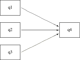
You can transcribe this path diagram into the following PATH model specification:
proc calis data=sales;
   path   q1 q2 q3 ===>  q4;
run;
In the path statement, the shorthand path specification
path q1 q2 q3 ===> q4;
is equivalent to the following specification:
   path   q1  ===>  q4,
          q2  ===>  q4,
          q3  ===>  q4;
The shorthand notation provides a more convenient way to specify the path model. Some of the model fit statistics are shown in Output 29.7.2. This is a saturated model with perfect fit and zero degrees of freedom. Because the chi-square statistic is always smallest in a saturated model (with a zero chi-square value), it does not makes much sense to judge the model quality solely by looking at the chi-square value. However, a saturated model is useful for serving as a baseline model with which other nonsaturated competing models are compared.
Output 29.7.2: Model Fit of the Multiple Regression Model for the Sales Data
In addition to the model fit chi-square statistic, Output 29.7.2 also shows Akaike’s information criterion (AIC), Bozdogan’s CAIC, and Schwarz’s Bayesian criterion (SBC) of the saturated
model. The AIC, CAIC, and SBC are derived from information theory and henceforth they are referred to as the information-theoretic
fit indices. These information-theoretic fit indices measure the model quality by taking the model parsimony into account.
The root mean square error of approximation (RMSEA) also takes the model parsimony into account, but it is not an information-theoretic
fit index. The values of these information-theoretic fit indices themselves do not indicate the quality of the model. However,
when you fit several different models to the same data, you can order the models by these fit indices. The better the model,
the smaller the fit index values. Unlike the chi-square statistic, these fit indices do not always favor a saturated model
because a saturated model lacks model parsimony (the saturated model uses the most parameters to explain the data). The subsequent
discussion uses these fit indices to select the "best" model for the sales data.
Output 29.7.3 shows the parameter estimates of the multiple regression model. In the first table, all path effect estimates are not statistically
significant—that is, all t values are less than 1.96. The next table in Output 29.7.3 shows the variance estimates of q1–q3 and the error variance estimate for q4. All of these estimates are significant. The last table in Output 29.7.3 shows the covariances among the exogenous variables q1–q3. These covariance estimates are small and are not statistically significant.
Output 29.7.3: Parameter Estimates of the Multiple Regression Model for the Sales Data
In Output 29.7.3, the total number of parameter estimates is 10 (_Parm1–_Parm3 and _Add1–_Add7). Under the covariance structure model, these 10 parameters explain the 10 nonredundant elements in the covariance matrix
for the sales data. That is why the model has a perfect fit with zero degrees of freedom.
In Output 29.7.3, notice that some parameters have the prefix '_Parm', while others have the prefix '_Add'. Both types of parameter names
are generated by PROC CALIS. The parameters named with the '_Parm' prefix are those that were specified in the model, but
were not named. In the current example, the parameters specified but not named are the path coefficients (effects) for the
three paths in the PATH statement. The parameters named with the '_Add' prefix are default parameters added by PROC CALIS.
In the current multiple regression example, the variances and covariances among the predictors (q1–q3) and the error variance for the outcome variable (q4) are default parameters in the model. In general, variances and covariances among exogenous variables and error variances
of endogenous variables are default parameters in the PATH model. Avoid using parameter names with the '_Parm' and '_Add'
prefixes to avoid confusion with parameters that are generated by PROC CALIS.
Direct and Indirect Effects Model for the Sales Data
In the multiple regression model, q1–q3 are all predictors that have direct effects on q4. This example considers the possibility of adding indirect effects into the multiple regression model. Because of the time
ordering, it is reasonable to assume that there is a causal sequence q1 ===> q2 ===> q3. To implement this idea into the model, put two more paths into the preceding path diagram to form the following new path
diagram:
Output 29.7.4:
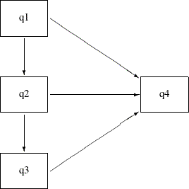
With the q1 ===> q2 and q2 ===> q3 paths, q2 and q3 are no longer exogenous in the model. They become endogenous. The only exogenous variable in the model is q1, which has a direct effect in addition to indirect effects on q4. The direct effect is indicated by the q1 ===> q4 path. The indirect effects are indicated by the following two causal chains: q1 ===> q2 ===> q4 and q1 ===> q2 ===> q3 ===> q4. Similarly, q2 has a direct and an indirect effect on q4. However, q3 has only a direct effect on q4. You can use the following statements to specify this direct and indirect effects model:
proc calis data=sales;
   path   q1       ===>  q2,
          q2       ===>  q3,
          q1 q2 q3 ===>  q4;
run;
Although the direct and indirect effects model has two more paths in the PATH statement than does the preceding multiple regression model, the current model is more
precise because it has one fewer parameter. By introducing the causal paths q1 ===> q2 and q2===> q3, the six variances and covariances among q1–q3 are explained by: the two causal effects, the exogenous variance of q1, and the error variances for q2 and q3 (that is, five parameters in the model). Hence, the current direct and indirect effects model has one fewer parameter than the preceding multiple regression model.
Output 29.7.5 shows some model fit indices of the direct and indirect effects model. The model fit chi-square is 0.0934 with one degree of freedom. It is not significant. Therefore, you cannot reject the model on statistical grounds. The standardized root mean squares of residuals (SRMR) is 0.028 and the root mean square error of approximation (RMSEA) is close to zero. Both indices point to a very good model fit. The AIC, CAIC, and SBC are all smaller than those of the saturated model, as shown in Output 29.7.2. This suggests that the direct and indirect effects model is better than the saturated model.
Output 29.7.5: Model Fit of the Direct and Indirect Effects Model for the Sales Data
Output 29.7.6 shows the parameter estimates of the direct and indirect effects model. All the path effects are not significant, while all the variance or error variance estimates are significant. Unlike
the saturated model where you have covariance estimates among several exogenous variables (as shown in Output 29.7.3), in the direct and indirect effects model there is only one exogenous variable (q1) and hence there is no covariance estimate in the results.
Output 29.7.6: Parameter Estimates of the Direct and Indirect Effects Model for the Sales Data
| PATH List | |||||||
|---|---|---|---|---|---|---|---|
| Path | Parameter | Estimate | Standard Error |
t Value | Pr > |t| | ||
| q1 | ===> | q2 | _Parm1 | 0.0005847 | 0.22602 | 0.00259 | 0.9979 |
| q2 | ===> | q3 | _Parm2 | 0.56323 | 0.42803 | 1.3159 | 0.1882 |
| q1 | ===> | q4 | _Parm3 | 0.55980 | 0.64705 | 0.8652 | 0.3870 |
| q2 | ===> | q4 | _Parm4 | 0.58946 | 0.84524 | 0.6974 | 0.4856 |
| q3 | ===> | q4 | _Parm5 | 0.88290 | 0.51450 | 1.7160 | 0.0862 |
Although the current direct and indirect effects model is better than the saturated model and both the SRMR and RMSEA indicate a good model fit, the nonsignificant path effect estimates are unsettling. You continue to explore alternative models for the data.
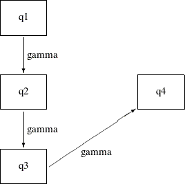
Indirect Effects Model for the Sales Data
The saturated model includes only the direct effects of q1–q3 on q4, while the direct and indirect effects model includes both the direct and indirect effects of q1 and q2 on q4. An alternative model with only the indirect effects of q1 and q2 on q4, but without their direct effects, is possible. Such an indirect effects model is represented by the following path diagram:
Output 29.7.7:
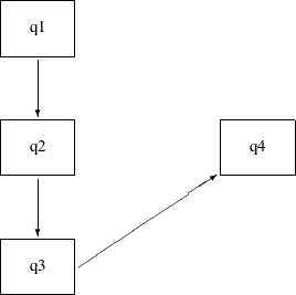
You can easily transcribe this path diagram into the following PATH model specification:
proc calis data=sales;
   path   q1   ===>  q2,
          q2   ===>  q3,
          q3   ===>  q4;
run;
Output 29.7.8 shows some model fit indices for the indirect effects model. The chi-square model fit statistic is not statistically significant, so the model is not rejected. The standardized RMR is 0.0905, which is a bit higher than the conventional value of 0.05 for an acceptable good model fit. However, the RMSEA is close to zero, which shows a very good model fit. The AIC, CAIC and SBC are all smaller than the direct and indirect effects model. These information-theoretic fit indices suggest that the indirect effects model is better.
Output 29.7.8: Model Fit of the Indirect Effects Model for the Sales Data
Output 29.7.9 shows the parameter estimates of the indirect effects model. All the variance and error variance estimates are statistically significant. However, only the path effect of q3 on q4 is statistically significant, and all other path effects are not. Having significant variances with nonsignificant paths
raises some concerns about accepting the current model even though the AIC, CAIC, and SBC values suggest that it is the best
model so far.
Output 29.7.9: Parameter Estimates of the Indirect Effects Model for the Sales Data
Constrained Indirect Effects Model for the Sales Data
In the preceding indirect effects model, some path effects are not significant. In the current model, all the path effects are constrained to be equal. The following path diagram represents the constrained indirect effects model:
Output 29.7.10:
Except for one notable difference, this path diagram is the same as the path diagram for the preceding indirect effects model. The current path diagram labels all the paths with the same name (gamma) to signify that they are the same parameter. You can specify this constrained indirect effects model with this chosen constraint on the path effects by the using following statements:
proc calis data=sales;
   path   q1   ===>  q2      = gamma,
          q2   ===>  q3      = gamma,
          q3   ===>  q4      = gamma;
run;
In the PATH statement, append an equal sign and a parameter name gamma in each of the path entries. This specification means that all the associated path effects are the same parameter named gamma.
Output 29.7.11 shows some fit indices for the constrained indirect effects model. Again, the model fit chi-square statistic is not significant. However, the SRMR is 0.2115, which is too large to accept as a good model. The RMSEA is 0.0499, which still indicates a good model fit. The AIC, CAIC, and SBC values are a bit smaller than those of the preceding unconstrained indirect effects model. Therefore, it seems that constraining the path effects leads to a slightly better model.
Output 29.7.11: Model Fit of the Constrained Indirect Effects Model for the Sales Data
Output 29.7.12 shows the parameter estimates of the constrained indirect effects model. Again, all variance and error variance estimates are significant, and all path effects are not significant. The effect
estimate is 0.24 (standard error=0.19, t = 1.25).
Output 29.7.12: Parameter Estimates of the Constrained Indirect Effects Model for the Sales Data
Constrained Indirect Effects and Error Variances Model for the Sales Data
In addition to constraining all the path effects in the preceding model, the current model constrains all the error variances. Before using a path diagram to represent the current constrained indirect effects and constrained error variances, it is important to realize that you have not manually defined variances and covariances in the path diagrams for all of the preceding models. The default parameterization in PROC CALIS defined those parameters.
Represent the variances and covariances in a path diagram with double-headed arrows. When a double-headed arrow points to
a single variable, it represents the variance parameter. When a double-headed arrow points to two distinct variables, it represents
the covariance between the two variables. Consider the unconstrained indirect effects model for the sales data as an example. A more complete path diagram representation is as follows:
Output 29.7.13:
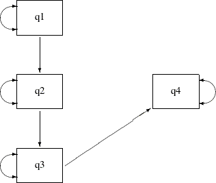
In this path diagram, a double-headed arrow on each variable represents variance or error variance. For q1, the double-headed arrow represents the variance parameter of q1. For other variables, the double-headed arrows represent error variances because those variables are endogenous (that is,
they are predicted from other variables) in the model.
In order to represent the equality-constrained parameters in the model, you can put parameter names in the respective parameter locations in the path diagram. For the current constrained indirect effects and error variances model, you can represent the model by the following path diagram:
Output 29.7.14:
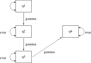
In the path diagram, label all the path effects by the parameter gamma and all error variances by the parameter evar. The double-headed arrow attached to q1 is not labeled by any name. This means that it is an unnamed free parameter in the model.
You can transcribe the path diagram into the following statements:
proc calis data=sales;
   path   q1   ===>  q2      = gamma,
          q2   ===>  q3      = gamma,
          q3   ===>  q4      = gamma;
   pvar   q2 q3 q4 = 3 * evar;
run;
The specification in the PATH statement is the same as the preceding PATH model specification for the constrained indirect effects model. The new specification here is the PVAR
statement. You use the PVAR statement to specify partial variances, which include the (total) variances of exogenous variables
and the error variances of the endogenous variables. In the PVAR statement, you specify the variables for which you intend
to define variances. If you do not specify anything after the list of variables, the variances of these variables are unnamed
free parameters. If you put an equal sign after the variable lists, you can specify parameter names, initial values, or fixed
parameters for the variances of the variables. See the PVAR
statement for details. In the current model, 3*evar means that you want to specify evar three times (for the error variance parameters of q2, q3, and q4).
Note that you did not specify the variance of q1 in the PVAR statement. This variance is a default parameter in the model, and therefore you do not need to specify it in
the PVAR statement. Alternatively, you can specify it explicitly in the PVAR statement by giving it a parameter name. For
example, you can specify the following:
pvar   q2 q3 q4 = 3 * evar,
       q1       = MyOwnName;
Or, you can specify it explicitly without giving it a parameter name, as shown in following statement:
pvar   q2 q3 q4 = 3 * evar,
       q1 ;
All these specifications lead to the same estimation results. The difference between the two specifications is the explicit
parameter name for the variance of q1. Without putting q1 in the PVAR statement, the variance parameter is named with the prefix _Add, which is generated as a default parameter by PROC CALIS. With the explicit specification of q1, the variance parameter is named MyOwnName. With the explicit specification of q1, but without giving it a parameter name in the PVAR statement, the variance parameter is named with the prefix _Parm, which PROC CALIS generates for unnamed free parameters.
Output 29.7.15 shows some fit indices for the constrained indirect effects and error variances model. The model fit chi-square is 19.7843, which is significant at the 0.05  -level. In practice, the model fit chi-square statistic is not the only criterion for judging model fit. In fact, it might
not even be the most commonly used criterion for measuring model fit. Other criteria such as the SRMR and RMSEA are more popular
or important. Unfortunately, the values of these two fit indices do not support the current constrained model either. The
SRMR is 1.5037 and the RMSEA is 0.3748. Both are much greater than the commonly accepted 0.05 criterion.
-level. In practice, the model fit chi-square statistic is not the only criterion for judging model fit. In fact, it might
not even be the most commonly used criterion for measuring model fit. Other criteria such as the SRMR and RMSEA are more popular
or important. Unfortunately, the values of these two fit indices do not support the current constrained model either. The
SRMR is 1.5037 and the RMSEA is 0.3748. Both are much greater than the commonly accepted 0.05 criterion.
Output 29.7.15: Model Fit of the Constrained Indirect Effects and Error Variances Model for the Sales Data
The AIC, CAIC, and SBC values are all much greater than those of the preceding constrained indirect effects model. Therefore, constraining the error variances in addition to the constrained indirect effects does not lead to a better model.
Output 29.7.16 shows the parameter estimates of the constrained indirect effects and error variances model. All estimates are significant in the model, which is often desirable. However, because of the bad model fit, this model is not acceptable.
Output 29.7.16: Parameter Estimates of the Constrained Indirect Effects and Error Variances Model for the Sales Data
Partially Constrained Model for the Sales Data
In the preceding model, constraining all error variances to be same shows that the model fit is unacceptable, even though all parameter estimates are significant. Relaxing those constraints a little might improve the model. The following path diagram represents such a partially constrained model:
Output 29.7.17:
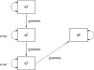
The only difference between the current partially constrained model and the preceding constrained indirect effects and error variances model is that the error variance for q4 is no longer constrained to be equal to the error variances of q2 and q3. In the path diagram, evar is no longer attached to the double-headed arrow that is associated with the error variance of q4. You can transcribe this path diagram representation into the following PATH model specification:
proc calis data=sales;
   path   q1   ===>  q2      = gamma,
          q2   ===>  q3      = gamma,
          q3   ===>  q4      = gamma;
   pvar   q2 q3 = 2 * evar,
          q4 q1;
run;
Now, the PVAR statement has only the error variances of q2 and q3 constrained to be equal. The error variance of q4 and the variance of q1 are free parameters without constraints.
Output 29.7.18 shows some fit indices for the partially constrained model. The chi-square model fit test statistic is not significant. The SRMR is 0.3877 and the RMSEA is 0.1164. These are far from the conventional acceptance level of 0.05. However, the AIC, CAIC, and SBC values are all slightly smaller than the constrained indirect effects model, as shown in Output 29.7.11. In fact, these information-theoretic fit indices suggest that the partially constrained model is the best model among all models that have been considered.
Output 29.7.18: Model Fit of the Partially Constrained Model for the Sales Data
Output 29.7.19 shows the parameter estimates of the partially constrained model. Again, all variance and error variance parameters are statistically significant. However, the path effects are only marginally significant.
Output 29.7.19: Parameter Estimates of the Partially Constrained Model for the Sales Data
Which Model Should You Choose?
You fit various models in this example for the sales data. The fit summary of the models is shown in the following table:
|
1 |
2 |
3 |
4 |
5 |
6 |
|
|---|---|---|---|---|---|---|
|
Constrained |
||||||
|
Direct and |
Constrained |
Indirect Effects |
||||
|
Indirect |
Indirect |
Indirect |
and Error |
Partially |
||
|
Saturated |
Effects |
Effects |
Effects |
Variances |
Constrained |
|
|
df |
0 |
1 |
3 |
5 |
7 |
6 |
|
p-value |
. |
0.76 |
0.74 |
0.40 |
0.01 |
0.32 |
|
SRMR |
0 |
0.03 |
0.09 |
0.21 |
1.50 |
0.39 |
|
RMSEA |
. |
0.00 |
0.00 |
0.05 |
0.37 |
0.12 |
|
AIC |
20.00 |
18.09 |
15.24 |
15.16 |
25.78 |
15.06 |
|
CAIC |
36.39 |
32.84 |
26.71 |
23.36 |
30.70 |
21.61 |
|
SBC |
26.39 |
23.84 |
19.71 |
18.36 |
27.70 |
17.61 |
As discussed previously, the model fit chi-square test statistic always favors models with a lot of parameters. It does not take model parsimony into account. In particular, a saturated model (Model 1) always has a perfect fit. However, it does not explain the data in a concise way. Therefore, the model fit chi-square statistic is not used here for comparing the competing models.
The standardized root mean square residual (SRMR) also does not take the model parsimony into account. It tells you how the fitted covariance matrix is different from the observed covariance matrix in a certain standardized way. Again, it always favors models with a lot of parameters. As shown in the preceding table, the more parameters (the fewer degrees of freedom) the model has, the smaller the SRMR is. A conventional criterion is to accept a model with SRMR less than 0.05. Applying this criterion, only the saturated model (Model 1) and the direct and indirect effects (Model 2) models are acceptable. The indirect effects model (Model 3) is marginally acceptable.
The root mean square error of approximation (RMSEA) fit index does take model parsimony into account. With the 'RMSEA less than 0.05 criterion', the constrained indirect effects and error variances model (Model 5) and the partially constrained model (Model 6) are not acceptable.
The information-theoretic fit indices such as the AIC, CAIC, and SBC also take model parsimony into account. All of these indices point to the partially constrained model (Model 6) as the best model among the competing models. However, because this model has a relatively bad absolute fit, as indicated by the large SRMR value (0.39), accepting this model is questionable. In addition, the information-theoretic fit indices of the indirect effects model (Model 3) and of the constrained indirect effects model (Model 4) are not too different from those of the partially constrained model (Model 6). The indirect effects model is especially promising because it has relatively small SRMR and RMSEA values. The drawback is that some path effect estimates in the indirect effects model are not significant. Perhaps collecting and analyzing more data might confirm these promising models with significant path effects.
You might not be able to draw a unanimous conclusion about the best model for the sales data of this example. Different fit indices in structural equation modeling do not always point to the same conclusions.
The analyses in the current example show some of the complexity of structural equation modeling. Some interesting questions
about model selections are:
-
Do you choose a model based on a single fit criterion? Or, do you consider a set of model fit criteria to weigh competing models?
-
Which fit index criterion is the most important for judging model fit?
-
In selecting your "best" model, how do you take "chance" into account?
-
How would you use your substantive theory to guide your model search?
The answers to these interesting research questions might depend on the context. Nonetheless, PROC CALIS can help you in the model selection process by computing various kinds of fit indices. (Only a few of these fit indices are shown in the output of this example. See the FITINDEX statement for a wide variety of fit indices that you can obtain from PROC CALIS.)
Alternative PATH Model Specifications for Variances and Covariances
The PATH modeling language of PROC CALIS is designed to map the path diagram representation into the PATH statement syntax efficiently. For any path that is denoted by a single-headed arrow in the path diagram, you can specify a path entry in the PATH statement. You can also specify double-headed arrows in the PATH statement.
Consider the preceding path diagram for the partially constrained model for the sales data. You use double-headed arrows to denote variances or error variances of the variables. The path diagram is shown in
the following:
Output 29.7.20:
As discussed previously, you can use the PVAR statement to specify these variances or error variances as in following syntax:
pvar   q2 q3 = 2 * evar,
       q4 q1;
Alternatively, you can specify these double-headed arrows directly as paths in the PATH statement, as shown in the following statements:
proc calis data=sales;
   path   q1   ===>  q2      = gamma,
          q2   ===>  q3      = gamma,
          q3   ===>  q4      = gamma,
          <==>    q2 q3      = 2 * evar,
          <==>    q4 q1;
run;
To specify the double-headed paths pointing to individual variables, you begin with the double-headed arrow notation <==>, followed by the list of variables. For example, in the preceding specification, the error variance of q4 and the variance of q1 are specified in the last path entry of the PATH statement. If you want to define the parameter names for the variances,
you can add a parameter list after an equal sign in the path entries. For example, the error variances of q2 and q3 are denoted by the free parameter evar in a path entry in the PATH statement.
Alternatively, you can specify the double-headed arrow paths literally in a PATH statement, as shown in the following equivalent specification:
proc calis data=sales;
   path   q1   ===>  q2      = gamma,
          q2   ===>  q3      = gamma,
          q3   ===>  q4      = gamma,
          q2   <==>  q2      = evar,
          q3   <==>  q3      = evar,
          q4   <==>  q4,
          q1   <==>  q1;
run;
For example, the path entry q1 <==> q1 specifies the variance of q1. It is an unnamed free parameter in the model.
Output 29.7.21 show the parameter estimates for this alternative specification method. All these estimates match exactly those with the PVAR statement specification, as shown in Output 29.7.19. The only difference is that all estimation results are now presented under one PATH List, as shown in Output 29.7.21, instead of as two tables as shown in Output 29.7.19.
Output 29.7.21: Path Estimates of the Partially Constrained Model for the Sales Data
| PATH List | |||||||
|---|---|---|---|---|---|---|---|
| Path | Parameter | Estimate | Standard Error |
t Value | Pr > |t| | ||
| q1 | ===> | q2 | gamma | 0.35546 | 0.18958 | 1.8750 | 0.0608 |
| q2 | ===> | q3 | gamma | 0.35546 | 0.18958 | 1.8750 | 0.0608 |
| q3 | ===> | q4 | gamma | 0.35546 | 0.18958 | 1.8750 | 0.0608 |
| q2 | <==> | q2 | evar | 0.40601 | 0.11261 | 3.6056 | 0.0003 |
| q3 | <==> | q3 | evar | 0.40601 | 0.11261 | 3.6056 | 0.0003 |
| q4 | <==> | q4 | _Parm1 | 2.29415 | 0.89984 | 2.5495 | 0.0108 |
| q1 | <==> | q1 | _Parm2 | 0.33830 | 0.13269 | 2.5495 | 0.0108 |
The double-headed arrow path syntax applies to covariance specification as well. For example, the following PATH statement
specifies the covariances among variables x1–x3:
path    x2 <==> x1,
        x3 <==> x1,
        x3 <==> x2;
In the beginning of the current example, you use the following path diagram to represent the multiple regression model for
the sales data:
Output 29.7.22:
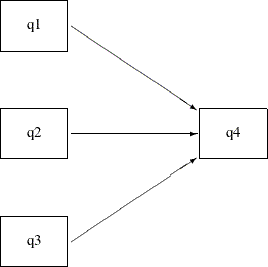
The following statements specify the multiple regression model:
proc calis data=sales;
   path   q1 q2 q3 ===>  q4;
run;
You do not represent the covariances and variances among the exogenous variables explicitly in the path diagram, nor in the PATH statement specification. However, PROC CALIS generates them as free parameters by default. Some researchers might prefer to represent the exogenous variances and covariances explicitly in the path diagram, as shown in the following path diagram:
Output 29.7.23:
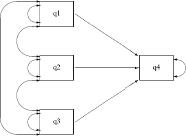
In the path diagram, there are three single-head arrows and seven double-headed arrows. These 10 paths represent the 10 parameters in the covariance structure model. To represent all these parameters in the PATH model specification, you can use the following statements:
proc calis data=sales;
   path   q1   ===>  q4  ,
          q2   ===>  q4  ,
          q3   ===>  q4  ,
          q1   <==>  q1  ,
          q2   <==>  q2  ,
          q3   <==>  q3  ,
          q1   <==>  q2  ,
          q2   <==>  q3  ,
          q1   <==>  q3  ,
          q4   <==>  q4  ;
run;
The first three path entries in the PATH statement reflect the single-headed paths in the path diagram. The next six path
entries in the PATH statement reflect the double-headed paths among the exogenous variables q1–q3 in the path diagram. The last path entry in the PATH statement reflects the double-headed path attached to the endogenous
variable q4 in the path diagram. With this specification, the parameter estimates for the multiple regression model are all shown in
Output 29.7.24.
Output 29.7.24: Path Estimates of the Multiple Regression Model for the Sales Data
| PATH List | |||||||
|---|---|---|---|---|---|---|---|
| Path | Parameter | Estimate | Standard Error |
t Value | Pr > |t| | ||
| q1 | ===> | q4 | _Parm01 | 0.55980 | 0.64938 | 0.8621 | 0.3887 |
| q2 | ===> | q4 | _Parm02 | 0.58946 | 0.84558 | 0.6971 | 0.4857 |
| q3 | ===> | q4 | _Parm03 | 0.88290 | 0.51635 | 1.7099 | 0.0873 |
| q1 | <==> | q1 | _Parm04 | 0.33830 | 0.13269 | 2.5495 | 0.0108 |
| q2 | <==> | q2 | _Parm05 | 0.22466 | 0.08812 | 2.5495 | 0.0108 |
| q3 | <==> | q3 | _Parm06 | 0.60633 | 0.23782 | 2.5495 | 0.0108 |
| q1 | <==> | q2 | _Parm07 | 0.0001978 | 0.07646 | 0.00259 | 0.9979 |
| q2 | <==> | q3 | _Parm08 | 0.12653 | 0.10821 | 1.1693 | 0.2423 |
| q1 | <==> | q3 | _Parm09 | 0.03610 | 0.12601 | 0.2865 | 0.7745 |
| q4 | <==> | q4 | _Parm10 | 1.84128 | 0.72221 | 2.5495 | 0.0108 |
These estimates are the same as those in Output 29.7.3, where the estimates are shown in three different tables, instead of in one table for all paths as in Output 29.7.24.
Sometimes, specification of some single-headed and double-headed paths can become very laborious. Fortunately, PROC CALIS provides shorthand notation for the PATH statement to make the specification more efficient. For example, a more concise way to specify the preceding multiple regression model is shown in the following statements:
proc calis data=sales;
   path   q1 q2 q3  ===>  q4  ,
          <==>  [q1-q3]  ,
          <==>  q4  ;
run;
The first path entry q1 q2 q3 ===> q4 in the PATH statement represents the three single-headed arrows in the path diagram. The second path entry <==> [q1-q3] generates the variances and covariances for the set of variables specified in the rectangular brackets. The last path entry
represents the error variance of q4. Consequently, expanding the preceding shorthand specification generates the following specification:
proc calis data=sales;
   path   q1   ===>  q4  ,
          q2   ===>  q4  ,
          q3   ===>  q4  ,
          q1   <==>  q1  ,
          q2   <==>  q1  ,
          q2   <==>  q2  ,
          q3   <==>  q1  ,
          q3   <==>  q2  ,
          q3   <==>  q3  ,
          q4   <==>  q4  ;
run;
Notice that the third through ninth path entries correspond to the lower triangular elements of the covariance matrix for
q1–q3.
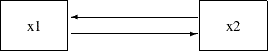
Caution: The double-headed path specification does not represent a reciprocal relationship. That is, the following statement specifies the covariance between x2 and x1:
path x2 <==> x1,
But the following statement specifies that x2 and x1 have reciprocal causal effects:
path    x2 <=== x1,
        x1 ===> x2;
The reciprocal causal effects specification reflects the following path diagram:
Output 29.7.25: