The CALIS Procedure
-
Overview

-
Getting Started
-
SyntaxClasses of Statements in PROC CALISSingle-Group Analysis SyntaxMultiple-Group Multiple-Model Analysis SyntaxPROC CALIS StatementBOUNDS StatementBY StatementCOSAN StatementCOV StatementDETERM StatementEFFPART StatementFACTOR StatementFITINDEX StatementFREQ StatementGROUP StatementLINCON StatementLINEQS StatementLISMOD StatementLMTESTS StatementMATRIX StatementMEAN StatementMODEL StatementMSTRUCT StatementNLINCON StatementNLOPTIONS StatementOUTFILES StatementPARAMETERS StatementPARTIAL StatementPATH StatementPATHDIAGRAM StatementPCOV StatementPVAR StatementRAM StatementREFMODEL StatementRENAMEPARM StatementSAS Programming StatementsSIMTESTS StatementSTD StatementSTRUCTEQ StatementTESTFUNC StatementVAR StatementVARIANCE StatementVARNAMES StatementWEIGHT Statement
-
DetailsInput Data SetsOutput Data SetsDefault Analysis Type and Default ParameterizationThe COSAN ModelThe FACTOR ModelThe LINEQS ModelThe LISMOD Model and SubmodelsThe MSTRUCT ModelThe PATH ModelThe RAM ModelNaming Variables and ParametersSetting Constraints on ParametersAutomatic Variable SelectionPath Diagrams: Layout Algorithms, Default Settings, and CustomizationEstimation CriteriaRelationships among Estimation CriteriaGradient, Hessian, Information Matrix, and Approximate Standard ErrorsCounting the Degrees of FreedomAssessment of FitCase-Level Residuals, Outliers, Leverage Observations, and Residual DiagnosticsLatent Variable ScoresTotal, Direct, and Indirect EffectsStandardized SolutionsModification IndicesMissing Values and the Analysis of Missing PatternsMeasures of Multivariate KurtosisInitial EstimatesUse of Optimization TechniquesComputational ProblemsDisplayed OutputODS Table NamesODS Graphics
-
ExamplesEstimating Covariances and CorrelationsEstimating Covariances and Means SimultaneouslyTesting Uncorrelatedness of VariablesTesting Covariance PatternsTesting Some Standard Covariance Pattern HypothesesLinear Regression ModelMultivariate Regression ModelsMeasurement Error ModelsTesting Specific Measurement Error ModelsMeasurement Error Models with Multiple PredictorsMeasurement Error Models Specified As Linear EquationsConfirmatory Factor ModelsConfirmatory Factor Models: Some VariationsResidual Diagnostics and Robust EstimationThe Full Information Maximum Likelihood MethodComparing the ML and FIML EstimationPath Analysis: Stability of AlienationSimultaneous Equations with Mean Structures and Reciprocal PathsFitting Direct Covariance StructuresConfirmatory Factor Analysis: Cognitive AbilitiesTesting Equality of Two Covariance Matrices Using a Multiple-Group AnalysisTesting Equality of Covariance and Mean Matrices between Independent GroupsIllustrating Various General Modeling LanguagesTesting Competing Path Models for the Career Aspiration DataFitting a Latent Growth Curve ModelHigher-Order and Hierarchical Factor ModelsLinear Relations among Factor LoadingsMultiple-Group Model for Purchasing BehaviorFitting the RAM and EQS Models by the COSAN Modeling LanguageSecond-Order Confirmatory Factor AnalysisLinear Relations among Factor Loadings: COSAN Model SpecificationOrdinal Relations among Factor LoadingsLongitudinal Factor Analysis
- References
Example 29.9 Testing Specific Measurement Error Models
In Example 29.8, you used the PATH modeling language of PROC CALIS to fit some basic measurement error models. In this example, you continue to fit the same kind of measurement error models but you restrict some model parameters to test some specific hypotheses.
This example uses the same data set as is used in Example 29.8. This data set contains 30 observations for the x and y variables. The general measurement error model with measurement errors in both x and y is shown in the following path diagram:
Output 29.9.1:
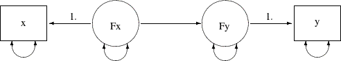
In the path diagram, two paths are fixed with a path coefficient of 1. They are required in the model for representing the relationships between true scores (latent) and measured indicators (observed). In Example 29.8, you consider several different modeling scenarios, all of which require you to make some parameter restrictions to estimate the models. You fix the measurement error variances to certain values that are based on prior knowledge or studies. Without those fixed error variances, those models would have been overparameterized and the parameters would not have been estimable.
For example, in the current path diagram, five of the single- or double-headed paths are not labeled with fixed numbers. Each
of these paths represents a free parameter in the model. However, in the covariance structure model analysis, you fit these
free parameters to the three nonredundant elements of the sample covariance matrix, which is a 2  2 symmetric matrix. Hence, to have an identified model, you can at most have three free parameters in your covariance structure
model. However, the path diagram shows that you have five free parameters in the model. You must introduce additional parameter
constraints to make the model identified.
2 symmetric matrix. Hence, to have an identified model, you can at most have three free parameters in your covariance structure
model. However, the path diagram shows that you have five free parameters in the model. You must introduce additional parameter
constraints to make the model identified.
If you do not have prior knowledge about the measurement error variances (as those described in Example 29.8), then you might need to make some educated guesses about how to restrict the overparameterized model. For example, if x and y are of the same kind of measurements, perhaps you can assume that they have an equal amount of measurement error variance.
Furthermore, if the measurement errors have been taken into account, in some physical science studies you might be able to
assume that the relationship between the true scores Fx and Fy is almost deterministic, resulting in a near zero error variance of Fy.
The assumptions here are not comparable to prior knowledge or studies about the measurement error variances. If you suppose they are reasonable enough in a particular field, you can use these assumptions to give you an identified model to work with (at least as an exploratory study) when the required prior knowledge is lacking. The following path diagram incorporates these two assumptions in the measurement error model:
Output 29.9.2:
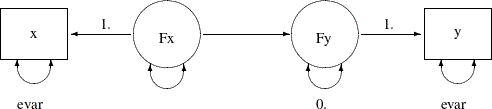
In the path diagram, you use evar to denote the error variances of x and y. This implicitly constrains the two error variances to be equal. The error variance of Fy is labeled zero, indicating a fixed parameter value and a deterministic relationship between x and y. You can transcribe this path diagram into the following PATH modeling specification:
proc calis data=measures;
   path
      x  <=== Fx  = 1.,
      Fx ===> Fy   ,
      Fy ===> y   = 1.;
   pvar
      x  = evar,
      y  = evar,
      Fy = 0.,
      Fx;
run;
In the PVAR statement, you specify the same parameter name evar for the error variances of x and y. This way their estimates are constrained to be the same in the estimation. In addition, the error variance for Fy is fixed at zero, which reflects the "near-deterministic" assumption about the relationship between Fx and Fy. These two assumptions effectively reduce the overparameterized model by two parameters so that the new model is just-identified
and estimable.
Output 29.9.3 shows the estimation results. The estimated effect of Fx on Fy is 1.3028 (standard error = 0.1134). The measurement error variances for x and y are both estimated at 0.0931 (standard error = 0.0244).
Output 29.9.3: Estimates of the Measurement Error Model with Equal Measurement Error Variances
Testing the Effect of Fx on Fy
Suppose you are interested in testing the hypothesis that the effect of Fx on Fy (that is, the regression slope) is 1. The following path diagram represents the model under the hypothesis:
Output 29.9.4:
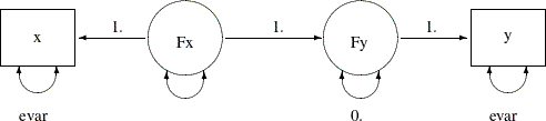
Now you label the path from Fx to Fy with a fixed constant 1, which reflects the hypothesis you want to test. You can transcribe the current path diagram easily
into the following PROC CALIS specification:
proc calis data=measures;
   path
      x  <=== Fx  = 1.,
      Fx ===> Fy  = 1.,  /* Testing a fixed constant effect */
      Fy ===> y   = 1.;
   pvar
      x  = evar,
      y  = evar,
      Fy = 0.,
      Fx;
run;
Output 29.9.5 shows the model fit chi-square statistic. The model fit chi-square test here essentially is a test of the null hypothesis of the constant effect at 1 because the alternative hypothesis is a saturated model. The chi-square value is 8.1844 (df = 1, p = .0042), which is statistically significant. This means that the hypothesis of constant effect at 1 is rejected.
Output 29.9.5: Fit Summary for Testing Constant Effect
Output 29.9.6 shows the estimates under this restricted model. In the first table of Output 29.9.6, all path effects or coefficients are fixed at 1. In the second tale of Output 29.9.6, estimates of the error variances are 0.1255 (standard error = 0.0330) for both x and y. The error variance of Fy is a fixed zero, as required in the hypothesis. The variance estimate of Fx is 0.9205 (standard error = 0.2587).
Output 29.9.6: Estimates of Constant Effect Measurement Error Model
Testing a Zero Intercept
Suppose you are interested in testing the hypothesis that the intercept for the regression of Fy on Fx is zero, while the regression effect is freely estimated. Because the intercept parameter belongs to the mean structures,
you need to specify this parameter in PROC CALIS to test the hypothesis.
There are two ways to include the mean structure analysis. First, you can include the MEANSTR option in the PROC CALIS statement. Alternatively, you can use the MEAN statement to specify the means and intercepts in the model. The following statements specify the model under the zero intercept hypothesis:
proc calis data=measures;
   path
      x  <=== Fx  = 1.,
      Fx ===> Fy  ,       /* regression effect is freely estimated */
      Fy ===> y   = 1.;
   pvar
      x  = evar,
      y  = evar,
      Fy = 0.,
      Fx;
   mean
      x y = 0. 0., /* Intercepts are zero in the measurement error model */
      Fy  = 0.,    /* Fixed to zero under the hypothesis */
      Fx;          /* Mean of Fx is freely estimated */
run;
In the PATH statement, the regression effect of Fx on Fy is freely estimated. In the MEAN statement, you specify the means or intercepts of the variables. Each variable in your measurement
error model has either a mean or an intercept (but not both) to specify. If a variable is exogenous (independent), you can
specify its mean in the MEAN statement. Otherwise, you can specify its intercept in the MEAN statement. Variables x and y in the measurement error model are both endogenous. They are measured indicators of their corresponding true scores Fx and Fy. Under the measurement error model, their intercepts are fixed zeros. The intercept for Fy is zero under the current hypothesized model. The mean of Fx is freely estimated under the model. This parameter is specified in the MEAN statement but is not named.
Output 29.9.7 shows the model fit chi-square statistic. The chi-square value is 10.5397 (df = 1, p = .0012), which is statistically significant. This means that the zero intercept hypothesis for the regression of Fy on Fx is rejected.
Output 29.9.7: Fit Summary for Testing Zero Intercept
Output 29.9.8 shows the estimates under the hypothesized model. The effect of Fx on Fy is 1.8169 (standard error = 0.0206). In the last table of Output 29.9.8, the estimate of the mean of Fx is 6.9048 (standard error = 0.1388). The intercepts for all other variables are fixed at zero under the hypothesized model.
Output 29.9.8: Estimates of the Zero Intercept Measurement Error Model
Measurement Model with Means and Intercepts Freely Estimated
In the preceding model, you fit a restricted regression model with a zero intercept. You reject the null hypothesis and conclude that this intercept is significantly different from zero. The alternative hypothesis is a saturated model with the intercept freely estimated. The model under the alternative hypothesis is specified in the following statements:
proc calis data=measures;
   path
      x  <=== Fx  = 1.,
      Fx ===> Fy  ,
      Fy ===> y   = 1.;
   pvar
      x  = evar,
      y  = evar,
      Fy = 0.,
      Fx;
   mean
      x y = 0. 0.,
      Fy Fx;
run;
Output 29.9.9 shows that model fit chi-square statistic is zero. This is expected because you are fitting a measurement error model with saturated mean and covariance structures.
Output 29.9.9: Fit Summary of the Saturated Measurement Model with Mean Structures
Output 29.9.10 shows the estimates under the measurement model with saturated mean and covariance structures. The effect of Fx on Fy is 1.3028 (standard error=0.1134), which is considerably smaller than the corresponding estimate in the restricted model
with zero intercept, as shown in Output 29.9.8. The intercept estimate of Fy is 3.5800 (standard error = 0.7864), with a significant t value of 4.55.
Output 29.9.10: Estimates of the Saturated Measurement Model with Mean Structures
In this example, you fit some measurement error models with some parameter constraints that reflect the hypothesized models of interest. You can set equality constraints by simply providing the same parameter names in the PATH model specification of PROC CALIS. You can also fix parameters to constants. In the MEAN statement, you can specify the intercepts and means of the variables in the measurement error models. You can apply all these techniques to more complicated measurement error models with multiple predictors, as shown in Example 29.10, where you also fit measurement error models with correlated errors.