The CALIS Procedure
-
Overview

-
Getting Started
-
SyntaxClasses of Statements in PROC CALISSingle-Group Analysis SyntaxMultiple-Group Multiple-Model Analysis SyntaxPROC CALIS StatementBOUNDS StatementBY StatementCOSAN StatementCOV StatementDETERM StatementEFFPART StatementFACTOR StatementFITINDEX StatementFREQ StatementGROUP StatementLINCON StatementLINEQS StatementLISMOD StatementLMTESTS StatementMATRIX StatementMEAN StatementMODEL StatementMSTRUCT StatementNLINCON StatementNLOPTIONS StatementOUTFILES StatementPARAMETERS StatementPARTIAL StatementPATH StatementPATHDIAGRAM StatementPCOV StatementPVAR StatementRAM StatementREFMODEL StatementRENAMEPARM StatementSAS Programming StatementsSIMTESTS StatementSTD StatementSTRUCTEQ StatementTESTFUNC StatementVAR StatementVARIANCE StatementVARNAMES StatementWEIGHT Statement
-
DetailsInput Data SetsOutput Data SetsDefault Analysis Type and Default ParameterizationThe COSAN ModelThe FACTOR ModelThe LINEQS ModelThe LISMOD Model and SubmodelsThe MSTRUCT ModelThe PATH ModelThe RAM ModelNaming Variables and ParametersSetting Constraints on ParametersAutomatic Variable SelectionPath Diagrams: Layout Algorithms, Default Settings, and CustomizationEstimation CriteriaRelationships among Estimation CriteriaGradient, Hessian, Information Matrix, and Approximate Standard ErrorsCounting the Degrees of FreedomAssessment of FitCase-Level Residuals, Outliers, Leverage Observations, and Residual DiagnosticsLatent Variable ScoresTotal, Direct, and Indirect EffectsStandardized SolutionsModification IndicesMissing Values and the Analysis of Missing PatternsMeasures of Multivariate KurtosisInitial EstimatesUse of Optimization TechniquesComputational ProblemsDisplayed OutputODS Table NamesODS Graphics
-
ExamplesEstimating Covariances and CorrelationsEstimating Covariances and Means SimultaneouslyTesting Uncorrelatedness of VariablesTesting Covariance PatternsTesting Some Standard Covariance Pattern HypothesesLinear Regression ModelMultivariate Regression ModelsMeasurement Error ModelsTesting Specific Measurement Error ModelsMeasurement Error Models with Multiple PredictorsMeasurement Error Models Specified As Linear EquationsConfirmatory Factor ModelsConfirmatory Factor Models: Some VariationsResidual Diagnostics and Robust EstimationThe Full Information Maximum Likelihood MethodComparing the ML and FIML EstimationPath Analysis: Stability of AlienationSimultaneous Equations with Mean Structures and Reciprocal PathsFitting Direct Covariance StructuresConfirmatory Factor Analysis: Cognitive AbilitiesTesting Equality of Two Covariance Matrices Using a Multiple-Group AnalysisTesting Equality of Covariance and Mean Matrices between Independent GroupsIllustrating Various General Modeling LanguagesTesting Competing Path Models for the Career Aspiration DataFitting a Latent Growth Curve ModelHigher-Order and Hierarchical Factor ModelsLinear Relations among Factor LoadingsMultiple-Group Model for Purchasing BehaviorFitting the RAM and EQS Models by the COSAN Modeling LanguageSecond-Order Confirmatory Factor AnalysisLinear Relations among Factor Loadings: COSAN Model SpecificationOrdinal Relations among Factor LoadingsLongitudinal Factor Analysis
- References
Example 29.12 Confirmatory Factor Models
This example shows how you can fit a confirmatory factor analysis model by the FACTOR modeling language. Thirty-two students
take tests of their verbal and math abilities. Six tests are administered separately. Tests x1–x3 test their verbal skills and tests y1–y3 test their math skills.
The data are shown in the following DATA step:
data scores;
   input x1 x2 x3 y1 y2 y3;
   datalines;
 23  17  16  15  14  16
 29  26  23  22  18  19
 14  21  17  15  16  18
 20  18  17  18  21  19
 25  26  22  26  21  26
 26  19  15  16  17  17
 14  17  19   4   6   7
 12  17  18  14  16  13
 25  19  22  22  20  20
  7  12  15  10  11   8
 29  24  30  14  13  16
 28  24  29  19  19  21
 12   9  10  18  19  18
 11   8  12  15  16  16
 20  14  15  24  23  16
 26  25  21  24  23  24
 20  16  19  22  21  20
 14  19  15  17  19  23
 14  20  13  24  26  25
 29  24  24  21  20  18
 26  28  26  28  26  23
 20  23  24  22  23  22
 23  24  20  23  22  18
 14  18  17  13  16  14
 28  34  27  25  21  21
 17  12  10  14  12  16
  8   1  13  14  15  14
 22  19  19  13  11  14
 18  21  18  15  18  19
 12  12  10  13  13  16
 22  14  20  20  18  19
 29  21  22  13  17  12
;
Because of the unambiguous nature of the tests, you hypothesize that this is a confirmatory factor model with two factors:
one is the verbal ability factor and the other is the math ability factor. You can represent such a confirmatory factor model by the following path diagram:
Output 29.12.1:
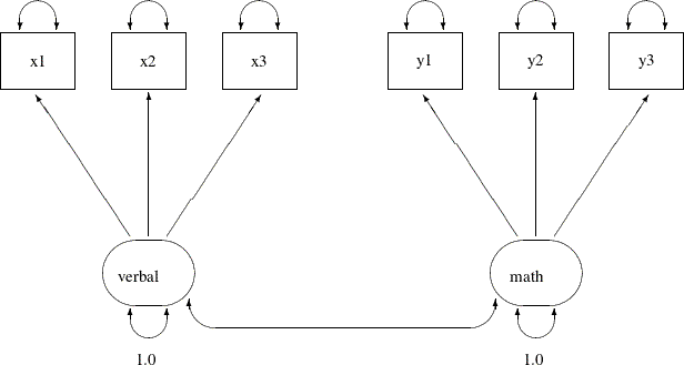
In the path diagram, there are two clusters of variables. One cluster is for the verbal factor and the other is for the math factor. The single-headed arrows in the path diagram represent functional relationships between factors and the observed
variables. The double-headed arrows that point to single variables represent variances of the factors or error variances of
the observed variables. The double-headed arrow that connect the two factors represents their covariance. All but two of these
arrows are not labeled with numbers. Each of the unlabeled arrows represents a free parameter in the confirmatory factor model.
You label the double-headed arrows that attach to the two factors with the constant 1. This means that the variances of the
factors are fixed at 1.0 in the model.
You can specify the confirmatory factor model by the FACTOR model language of PROC CALIS, as shown in the following statements:
proc calis data=scores;
   factor
      verbal ===> x1-x3,
      math   ===> y1-y3;
   pvar
      verbal = 1.,
      math   = 1.;
run;
In each of the entry of the FACTOR statement, you specify a latent factor, followed by a list of observed variables that are
functionally related to the latent factor. For example, in the first entry, the verbal factor is related to variables x1–x3, as shown by the single-headed arrows in the path diagram. In fact, all single-headed arrows in the path diagram are specified
in the FACTOR statement. Notice that each entry of the FACTOR statement must take the format of
factor_name ===> variable_list
You cannot reverse the arrow specification as in the following:
variable_list <=== factor_name
Nor you can have a specification such as the following:
variable_list ===> factor_name
However, you can specify the functional relationships between factors and variables in different entries. For example, you can specify the same confirmatory factor model by the following statements:
title "Basic Confirmatory Factor Model: Separate Path Entries";
title2 "FACTOR Model Specification";
proc calis data=scores;
   factor
      verbal ===> x1,
      verbal ===> x2,
      verbal ===> x3,
      math   ===> y1,
      math   ===> y2,
      math   ===> y3;
   pvar
      verbal = 1.,
      math   = 1.;
   fitindex  noindextype on(only)=[chisq df probchi rmsea  srmr bentlercfi];
run;
In the PVAR statement, which is for the specification of variances or error variances, you fix the variances of the latent
factors to 1. This completes the model specification of the confirmatory factor model, although you do not specify other arrows
in the path diagram as free parameters in these statements. The reason is that in the FACTOR modeling language, the variances
and covariances among factors and the error variances of the observed variables are default parameters in the confirmatory
factor model. It is not necessary to specify these parameters (or the corresponding arrows in the path diagram) explicitly
if they are free parameters in the model. You can also specify these free parameters explicitly without affecting the estimation.
However, if these parameters (or the corresponding double-headed arrows in the path diagram) are intended to be constrained
parameters or fixed values, you must specify them explicitly. For example, in the current confirmatory factor model, you must
provide explicit specifications for the variances of the verbal and the math factors because these parameters are fixed at 1.
Output 29.12.2 shows the modeling information and the variables in the confirmatory factor model.
Output 29.12.2: Modeling Information and Variables of the CFA Model: Scores Data
In the beginning of the output, PROC CALIS shows the data set, the number of observations, the model type, and the analysis type. The default analysis type in PROC CALIS is covariances (that is, covariance structures). If you want to analyze the correlation structures instead, you can use the CORR option in the PROC CALIS statement. Next, PROC CALIS shows the list of variables and factors in the model. As expected, the number of variables is 6 and the number of factors is 2.
Output 29.12.3 shows the initial model specifications of the confirmatory factor model.
Output 29.12.3: Initial Specification of the CFA Model: Scores Data
The first table of Output 29.12.3 shows the pattern of factor loadings of the variables on the two latent factors. As expected, x1–x3 have nonzero loadings only on the verbal factor, while y1–y3 have nonzero loadings on the math factor. PROC CALIS names these free parameters automatically with the "_Parm" prefix and unique numerical suffixes. There
are six parameters in the factor loading matrix with six different parameter names.
The next table of Output 29.12.3 shows the covariance matrix of the factors. The variances of the factors are fixed at one, as shown on the diagonal of the
covariance matrix. The covariance between the two factors is a free parameter named _Add1. You did not specify this covariance parameter explicitly in the factor model specification. By default, PROC CALIS assumes
that latent factors are correlated. Default free parameters added by PROC CALIS have the _Add prefix for their names. If you do not want to assume the covariances among the factors, you must specify zero covariances
in the COV statement. For example, the following statement specifies that the math and verbal factors have zero covariance:
 COV
   math verbal = 0.;
The last table of Output 29.12.3 shows the error variance parameters of the observed variables. By default PROC CALIS assumes these error variances are free
parameters in the confirmatory factor model. These added parameters are named with the _Add prefix. However, as all other default parameters that are assumed by PROC CALIS, you can overwrite the default by using explicit
specifications. You can specify the error variances of a confirmatory factor model explicitly in the PVAR statement. See specifications
in Example 29.13.
Output 29.12.4 shows the fit summary of the confirmatory factor model for the scores data.
Output 29.12.4: Fit Summary of the CFA Model: Scores Data
The model fit chi-square is 9.805 (df = 8, p = 0.279). This shows that statistically you cannot reject the confirmatory factor model for the test scores. However, the root mean square error of approximation (RMSEA) estimate is 0.0853, which is greater than the conventional 0.05 value for a good model fit. The standardized root mean square residual (SRMR) is 0.0571, which is close to the conventional 0.05 value for a good model fit. Bentler’s comparative fit index is 0.9887, which indicates a very good model fit. Overall, the model seems to be quite reasonable for the data.
Output 29.12.5 shows the loading and factor covariance estimates of the confirmatory factor model for the scores data. The first table shows the loading estimates, together with the standard error estimates and the t values. In structural equation modeling, the significance of the parameter estimates is usually inferred by comparing the
t values with the critical value of a standardized normal variate (that is, the z-table). Therefore, estimates with associated (absolute) t values greater than 1.96 are significant at  =.05. In Output 29.12.5, all the t values for the loading estimates are greater than 2. This indicates that the prescribed relationships between the variables
and the factors are significant.
=.05. In Output 29.12.5, all the t values for the loading estimates are greater than 2. This indicates that the prescribed relationships between the variables
and the factors are significant.
Output 29.12.5: Loading and Factor Covariance Estimates of the CFA Model: Scores Data
| Factor Loading Matrix: Estimate/StdErr/t-value/p-value | ||||||||||||
|---|---|---|---|---|---|---|---|---|---|---|---|---|
| verbal | math | |||||||||||
| x1 |
|
|
||||||||||
| x2 |
|
|
||||||||||
| x3 |
|
|
||||||||||
| y1 |
|
|
||||||||||
| y2 |
|
|
||||||||||
| y3 |
|
|
||||||||||
The second table of Output 29.12.5 shows the covariance matrix of the verbal and the math factors. Because the factor variances are fixed at one, the covariance estimate is also the correlation between the two factors.
Output 29.12.5 shows that the two factors are moderately correlated with a correlation estimate of 0.5175, which is statistically significant.
Output 29.12.6 shows the estimates of the error variances. All but the error variance of y1 are significant. This suggests that y1 might have an almost perfect relationship with the math factor.
Output 29.12.6: Error Variance Estimates of the CFA Model: Scores Data
| Error Variances | |||||
|---|---|---|---|---|---|
| Variable | Parameter | Estimate | Standard Error |
t Value | Pr > |t| |
| x1 | _Add2 | 11.52376 | 4.26398 | 2.7026 | 0.0069 |
| x2 | _Add3 | 9.14503 | 3.83219 | 2.3864 | 0.0170 |
| x3 | _Add4 | 6.68169 | 2.59770 | 2.5722 | 0.0101 |
| y1 | _Add5 | 0.78580 | 1.29440 | 0.6071 | 0.5438 |
| y2 | _Add6 | 2.88069 | 1.09395 | 2.6333 | 0.0085 |
| y3 | _Add7 | 5.15573 | 1.46854 | 3.5108 | 0.0004 |
Output 29.12.7 echoes this same fact. The R-squares in this table shows the percentages of variance of the variables that are overlapped
with the factors. While all these percentages (0.74 – 0.97) are quite high for all variables, the percentage is especially
high for y1. It shares 97% of the variance with the math factor. So, it appears that the observed variable y1 is almost a perfect indicator of the math factor.
Output 29.12.7: Squared Multiple Correlations of the CFA Model: Scores Data
Alternative Identification Constraints
Setting the variances of the latent factors to 1 in the preceding FACTOR model specification makes the model identified. This is necessary because the scales of the latent factors are arbitrary and the constraints imposed on the factor variances fix the scales of the factors.
In practice, there is another way to fix the scales of the factors. For each factor, you can fix the loading of one of its
measured indicators to a constant. This fixed loading value is usually set at 1. For example, you can represent the confirmatory
factor model for the scores data by the following alternative path diagram:
Output 29.12.8:
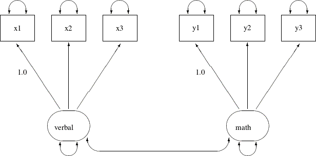
This path diagram is essentially the same as the preceding one. However, the fixed constants adjacent to the double-headed arrows that attach to the two factors in the preceding path diagram are now moved to two of the single-headed paths in the current path diagram.
You can specify this path diagram by the following FACTOR model specification of PROC CALIS:
ods graphics on;
proc calis data=scores plots=pathdiagram;
   factor
      verbal ===> x1-x3   = 1. ,
      math   ===> y1-y3   = 1. ;
run;
ods graphics off;
The PLOTS=PATHDIAGRAM option requests the path diagram output. In the FACTOR statement, you assign a fixed constant to each
of the path entries. In the first entry, the constant 1 is assigned to the loading of x1 on the verbal factor, while all other loadings in this entry are (unnamed) free parameters. Similarly, in the second entry, the fixed constant
1 is assigned to the loading of y1 on the math factor, while all other loadings in this entry are (unnamed) free parameters. This completes the specification of the confirmatory
factor model because all the double-headed arrows in the path diagram correspond to default free parameters in the FACTOR
modeling language of PROC CALIS.
Output 29.12.9 shows some fit indices for the current confirmatory factor model for the scores data.
Output 29.12.9: Fit Summary of the CFA Model with Alternative Identification Constraints: Scores Data
The model fit chi-square is 9.805 (df = 8, p = 0.279). This is the same model fit chi-square as that for the preceding CFA model specification with factor variances constrained to 1. In fact, all fit information in Output 29.12.9 are identical to Output 29.12.4.
Output 29.12.10 shows the path diagram of the confirmatory factor model. The path diagram indicates significant estimates by attaching asterisks
to the numerical values. Estimates that are flagged with one asterisk are significant at 0.05 -level. Estimates that are flagged with two asterisks are significant at 0.01 -level. The path diagram also shows a summary of fit statistics. For more information about specifying path diagram output,
see the section Path Diagrams: Layout Algorithms, Default Settings, and Customization.
Output 29.12.10: Path Diagram and Fit Summary: Scores Data
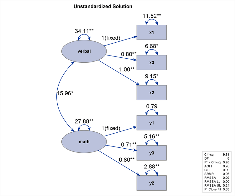
Output 29.12.11 shows the parameter estimates under the current model specification. The loading of x1 on the verbal factor is a fixed at 1, as required for the identification of the scale of the verbal factor. Similarly, the loading of y1 on the math factor is a fixed at 1 for the identification of the scale of the math factor. All other loading estimates in Output 29.12.11 are not the same as those in the preceding model specification, as shown in Output 29.12.5. The reason is that the scales of the factors (as measured by the estimated standard deviations of the factors) in the two
specifications are not the same. In the current model specification, the verbal factor has an estimated variance of 34.1123 and the math factor has an estimated variance of 27.8825, as shown in the second table of Output 29.12.11. Hence, the estimated standard deviations of these two factors are 5.8406 and 5.2804, respectively. But the standard deviations
of the factors in the preceding confirmatory factor model specification are fixed at 1.
Output 29.12.11: Loading and Factor Covariance Estimates of the CFA Model with Alternative Identification Constraints: Scores Data
However, if you multiply the loading estimates in Output 29.12.11 by the corresponding estimated factor standard deviation, you get the same set of loading estimates as in Output 29.12.5. For example, the loading of x1 on the verbal factor is 1.0 in Output 29.12.11. Multiplying this loading by the estimated standard deviation 5.8406 of the verbal factor gives you the same corresponding loading as in Output 29.12.5. Another example is the loading of y3 on the math factor. This loading is 0.7120 in Output 29.12.11. Multiplying this estimate by the estimated standard deviation 5.2804 of the verbal factor gives an estimate of 3.7596, which matches the corresponding loading estimate in Output 29.12.5. Therefore, the discrepancies in the loading estimates are due to different factor scales in the two specifications. The
loading estimates in Output 29.12.11 are simply rescaled version of the loading estimates in Output 29.12.5.
However, the scales of the factors do not affect the estimates of the error variances, as shown in Output 29.12.12. These estimates are the same as those for the preceding model specification, as shown in the Output 29.12.6.
Output 29.12.12: Error Variance Estimates of the CFA Model with Alternative Identification Constraints: Scores Data
| Error Variances | |||||
|---|---|---|---|---|---|
| Variable | Parameter | Estimate | Standard Error |
t Value | Pr > |t| |
| x1 | _Add4 | 11.52376 | 4.26398 | 2.7026 | 0.0069 |
| x2 | _Add5 | 9.14503 | 3.83219 | 2.3864 | 0.0170 |
| x3 | _Add6 | 6.68169 | 2.59770 | 2.5722 | 0.0101 |
| y1 | _Add7 | 0.78580 | 1.29440 | 0.6071 | 0.5438 |
| y2 | _Add8 | 2.88069 | 1.09395 | 2.6333 | 0.0085 |
| y3 | _Add9 | 5.15573 | 1.46854 | 3.5108 | 0.0004 |
This example shows how you can fit a basic confirmatory factor model by the FACTOR modeling language of PROC CALIS. You can
set the identification constraints and get statistically equivalent estimation results in two different ways. By setting up
additional parameter constraints, you can also fit some variations of the basic confirmatory factor model. See Example 29.13 for illustrations of some restricted confirmatory factor models for the scores data.
When your data have missing values, with the default ML estimation method PROC CALIS deletes all observations with missing
values for the analysis. This might result in a serious loss of information. Example 29.15 considers a hypothetical situation where some observations in the scores data have missing values in the observed variables. Only 16 observations have complete data. By using the full information
maximum likelihood (FIML) method for treating the missing data, Example 29.15 shows how you can fully use the information from the scores data set with missing values.