The CALIS Procedure
-
Overview

-
Getting Started
-
SyntaxClasses of Statements in PROC CALISSingle-Group Analysis SyntaxMultiple-Group Multiple-Model Analysis SyntaxPROC CALIS StatementBOUNDS StatementBY StatementCOSAN StatementCOV StatementDETERM StatementEFFPART StatementFACTOR StatementFITINDEX StatementFREQ StatementGROUP StatementLINCON StatementLINEQS StatementLISMOD StatementLMTESTS StatementMATRIX StatementMEAN StatementMODEL StatementMSTRUCT StatementNLINCON StatementNLOPTIONS StatementOUTFILES StatementPARAMETERS StatementPARTIAL StatementPATH StatementPATHDIAGRAM StatementPCOV StatementPVAR StatementRAM StatementREFMODEL StatementRENAMEPARM StatementSAS Programming StatementsSIMTESTS StatementSTD StatementSTRUCTEQ StatementTESTFUNC StatementVAR StatementVARIANCE StatementVARNAMES StatementWEIGHT Statement
-
DetailsInput Data SetsOutput Data SetsDefault Analysis Type and Default ParameterizationThe COSAN ModelThe FACTOR ModelThe LINEQS ModelThe LISMOD Model and SubmodelsThe MSTRUCT ModelThe PATH ModelThe RAM ModelNaming Variables and ParametersSetting Constraints on ParametersAutomatic Variable SelectionPath Diagrams: Layout Algorithms, Default Settings, and CustomizationEstimation CriteriaRelationships among Estimation CriteriaGradient, Hessian, Information Matrix, and Approximate Standard ErrorsCounting the Degrees of FreedomAssessment of FitCase-Level Residuals, Outliers, Leverage Observations, and Residual DiagnosticsLatent Variable ScoresTotal, Direct, and Indirect EffectsStandardized SolutionsModification IndicesMissing Values and the Analysis of Missing PatternsMeasures of Multivariate KurtosisInitial EstimatesUse of Optimization TechniquesComputational ProblemsDisplayed OutputODS Table NamesODS Graphics
-
ExamplesEstimating Covariances and CorrelationsEstimating Covariances and Means SimultaneouslyTesting Uncorrelatedness of VariablesTesting Covariance PatternsTesting Some Standard Covariance Pattern HypothesesLinear Regression ModelMultivariate Regression ModelsMeasurement Error ModelsTesting Specific Measurement Error ModelsMeasurement Error Models with Multiple PredictorsMeasurement Error Models Specified As Linear EquationsConfirmatory Factor ModelsConfirmatory Factor Models: Some VariationsResidual Diagnostics and Robust EstimationThe Full Information Maximum Likelihood MethodComparing the ML and FIML EstimationPath Analysis: Stability of AlienationSimultaneous Equations with Mean Structures and Reciprocal PathsFitting Direct Covariance StructuresConfirmatory Factor Analysis: Cognitive AbilitiesTesting Equality of Two Covariance Matrices Using a Multiple-Group AnalysisTesting Equality of Covariance and Mean Matrices between Independent GroupsIllustrating Various General Modeling LanguagesTesting Competing Path Models for the Career Aspiration DataFitting a Latent Growth Curve ModelHigher-Order and Hierarchical Factor ModelsLinear Relations among Factor LoadingsMultiple-Group Model for Purchasing BehaviorFitting the RAM and EQS Models by the COSAN Modeling LanguageSecond-Order Confirmatory Factor AnalysisLinear Relations among Factor Loadings: COSAN Model SpecificationOrdinal Relations among Factor LoadingsLongitudinal Factor Analysis
- References
Total, Direct, and Indirect Effects
Most structural equation models involve the specification of the effects of variables on each other. Whenever you specify equations in the LINEQS model, paths in the PATH model, path coefficient parameters in the RAM model, variable-factor relations in the FACTOR model, or regression coefficients in model matrices of the LISMOD model, you are specifying direct effects of predictor variables on outcome variables. All direct effects are represented by the associated regression coefficients, either fixed or free, in the specifications. You can examine the direct effect estimates easily in the output for model estimation.
However, direct effects are not the only effects that are important. In some cases, the indirect effects or total effects are of interest too. For example, suppose Self-Esteem is an important factor of Job Performance in your theory. Although it does not have a direct effect on Job Performance , it affects Job Performance through its influences on Motivation and Endurance. Also, Motivation has a direct effect on Endurance in your theory. The following path diagram summarizes such a theory:
Figure 29.25: Direct and Indirect Effects of Self-Esteem on Job Performance
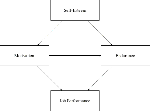
Clearly, each path in the diagram represents a direct effect of a predictor variable on an outcome variable. Less apparent are the total and indirect effects implied by the same path diagram. Despite this, interesting theoretical questions regarding the total and indirect effects can be raised in such a model. For example, even though there is no direct effect of Self-Esteem on Job Performance, what is its indirect effect on Job Performance? In addition to its direct effect on Job Performance, Motivation also has an indirect effect on Job Performance via its effect on Endurance. So, what is the total effect of Motivation on Job Performance and what portion of this total effect is indirect? The TOTEFF option of the CALIS statement and the EFFPART statement are designed to address these questions. By using the TOTEFF option or the EFFPART statement, PROC CALIS can compute the total, direct, and indirect effects of any sets of predictor variables on any sets of outcome variables. In this section, formulas for computing these effects are presented.
Formulas for Computing Total, Direct and Indirect Effects
No matter which modeling language is used, variables in a model can be classified into three groups. The first group is the so-called dependent variables, which serve as outcome variables at least once in the model. The other two groups consist of the remaining independent variables, which never serve as outcome variables in the model. The second group consists of independent variables that are unsystematic sources such as error and disturbance variables. The third group consists of independent variables that are systematic sources only.
Any variable, no matter which group it falls into, can have effects on the first group of variables. By definition, however, effects of variables in the first group on the other two groups do not exist. Because the effects of unsystematic sources in the second group are treated as residual effects on the first group of dependent variables, these effects are trivial in the sense that they always serve as direct effects only. That is, the effects from the second group of unsystematic sources partition trivially—total effects are always the same as the direct effects for this group. Therefore, for the purpose of effect analysis or partitioning, only the first group (dependent variables) and the third group (systematic independent variables) are considered.
Define  to be the set of
  dependent variables in the first group and w to be the set of
  systematic independent variables in the third group. Variables in both groups can be manifest or latent. All variables in
the effect analysis is thus represented by the vector
systematic independent variables in the third group. Variables in both groups can be manifest or latent. All variables in
the effect analysis is thus represented by the vector  .
.
The  matrix
  of direct effects refers to the path coefficients from all column variables to the row variables. This matrix is represented by:
![\[ \mb{D} = \left( \begin{array}{cc} \bbeta & \bgamma \\ \mb{0} & \mb{0} \\ \end{array} \right) \]](images/statug_calis0824.png)
where  is an
is an  matrix for direct effects of dependent variables on dependent variables and
  is an
is an  matrix for direct effects of systematic independent variables on dependent variables. By definition, there should not be
any direct effects on independent variables, and therefore the lower submatrices of are null. In addition, by model restrictions the diagonal elements of matrix must be zeros.
matrix for direct effects of systematic independent variables on dependent variables. By definition, there should not be
any direct effects on independent variables, and therefore the lower submatrices of are null. In addition, by model restrictions the diagonal elements of matrix must be zeros.
Correspondingly, the matrix  of total effects of column variables on the row variables is computed by:
![\[ \mb{T} = \left( \begin{array}{cc} (\bI -\bbeta )^{-1}-\bI & (\bI -\bbeta )^{-1}\bgamma \\ \mb{0} & \mb{0} \\ \end{array} \right) \]](images/statug_calis0828.png)
Finally, the matrix  of indirect effects of column variables on the row variables is computed by the difference between and as:
![\[ \bmu = \left( \begin{array}{cc} (\bI -\bbeta )^{-1}-\bI -\bbeta & (\bI -\bbeta )^{-1}\bgamma -\bgamma \\ \mb{0} & \mb{0} \\ \end{array} \right) \]](images/statug_calis0829.png)
In PROC CALIS, any subsets of , , and can be requested via the specification in the EFFPART
statement. All you need to do is to specify the sets of column variables (variables that have effects on others) and row
variables (variables that receive the effects, direct or indirect). Specifications of the column and row variables are done
conveniently by specifying variable names—no matrix terminology is needed. This feature is very handy if you have some focused
subsets of effects that you want to analyze a priori. See the
EFFPART statement
for details about specifications.
Stability Coefficient of Reciprocal Causation
For recursive models (that is, models without cyclical paths of effects), using the preceding formulas for computing the total effect and the indirect effect is appropriate without further restrictions. However, for non-recursive models (that is, models with reciprocal effects or cyclical effects) the appropriateness of the preceding formulas for effect computations is restricted to situations with the convergence of the total effects.
A necessary and sufficient condition for the convergence of total effects (with or without cyclical paths) is when all eigenvalues,
complex or real, of the matrix fall into a unit circle (see Bentler and Freeman 1983). Equivalently, define the stability coefficient of reciprocal causation as the largest length (modulus) of the eigenvalues
of the matrix. A stability coefficient less than one would ensure that all eigenvalues, complex or real, of the matrix fall into a unit circle. Hence, stability coefficient that is less than one is a necessary and sufficient condition
for the convergence of the total effects, which in turn substantiates the appropriateness of total and indirect effect computations.
Whenever effect analysis or partitioning is requested, PROC CALIS will check the appropriateness of effect computations by
evaluating the stability coefficient of reciprocal causation. If the stability coefficient is greater than one, computations
of the total and indirect effects will not be done.