The CALIS Procedure
-
Overview

-
Getting Started
-
SyntaxClasses of Statements in PROC CALISSingle-Group Analysis SyntaxMultiple-Group Multiple-Model Analysis SyntaxPROC CALIS StatementBOUNDS StatementBY StatementCOSAN StatementCOV StatementDETERM StatementEFFPART StatementFACTOR StatementFITINDEX StatementFREQ StatementGROUP StatementLINCON StatementLINEQS StatementLISMOD StatementLMTESTS StatementMATRIX StatementMEAN StatementMODEL StatementMSTRUCT StatementNLINCON StatementNLOPTIONS StatementOUTFILES StatementPARAMETERS StatementPARTIAL StatementPATH StatementPATHDIAGRAM StatementPCOV StatementPVAR StatementRAM StatementREFMODEL StatementRENAMEPARM StatementSAS Programming StatementsSIMTESTS StatementSTD StatementSTRUCTEQ StatementTESTFUNC StatementVAR StatementVARIANCE StatementVARNAMES StatementWEIGHT Statement
-
DetailsInput Data SetsOutput Data SetsDefault Analysis Type and Default ParameterizationThe COSAN ModelThe FACTOR ModelThe LINEQS ModelThe LISMOD Model and SubmodelsThe MSTRUCT ModelThe PATH ModelThe RAM ModelNaming Variables and ParametersSetting Constraints on ParametersAutomatic Variable SelectionPath Diagrams: Layout Algorithms, Default Settings, and CustomizationEstimation CriteriaRelationships among Estimation CriteriaGradient, Hessian, Information Matrix, and Approximate Standard ErrorsCounting the Degrees of FreedomAssessment of FitCase-Level Residuals, Outliers, Leverage Observations, and Residual DiagnosticsLatent Variable ScoresTotal, Direct, and Indirect EffectsStandardized SolutionsModification IndicesMissing Values and the Analysis of Missing PatternsMeasures of Multivariate KurtosisInitial EstimatesUse of Optimization TechniquesComputational ProblemsDisplayed OutputODS Table NamesODS Graphics
-
ExamplesEstimating Covariances and CorrelationsEstimating Covariances and Means SimultaneouslyTesting Uncorrelatedness of VariablesTesting Covariance PatternsTesting Some Standard Covariance Pattern HypothesesLinear Regression ModelMultivariate Regression ModelsMeasurement Error ModelsTesting Specific Measurement Error ModelsMeasurement Error Models with Multiple PredictorsMeasurement Error Models Specified As Linear EquationsConfirmatory Factor ModelsConfirmatory Factor Models: Some VariationsResidual Diagnostics and Robust EstimationThe Full Information Maximum Likelihood MethodComparing the ML and FIML EstimationPath Analysis: Stability of AlienationSimultaneous Equations with Mean Structures and Reciprocal PathsFitting Direct Covariance StructuresConfirmatory Factor Analysis: Cognitive AbilitiesTesting Equality of Two Covariance Matrices Using a Multiple-Group AnalysisTesting Equality of Covariance and Mean Matrices between Independent GroupsIllustrating Various General Modeling LanguagesTesting Competing Path Models for the Career Aspiration DataFitting a Latent Growth Curve ModelHigher-Order and Hierarchical Factor ModelsLinear Relations among Factor LoadingsMultiple-Group Model for Purchasing BehaviorFitting the RAM and EQS Models by the COSAN Modeling LanguageSecond-Order Confirmatory Factor AnalysisLinear Relations among Factor Loadings: COSAN Model SpecificationOrdinal Relations among Factor LoadingsLongitudinal Factor Analysis
- References
Example 29.15 The Full Information Maximum Likelihood Method
This example shows how you can fully utilize all available information from the data when there is a high proportion of observations with random missing value. You use the full information maximum likelihood method for model estimation.
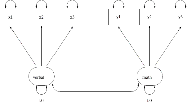
In Example 29.12, 32 students take six tests. These six tests are indicator measures of two ability factors: verbal and math. You conduct a confirmatory factor analysis in Example 29.12 based on a data set without any missing values. The path diagram for the confirmatory factor model is shown the following:
Output 29.15.1:
Suppose now due to sickness or unexpected events, some students cannot take part in one of these tests. Now, the data test contains missing values at various locations, as indicated by the following DATA step:
data missing;
   input x1 x2 x3 y1 y2 y3;
   datalines;
 23   .  16  15  14  16
 29  26  23  22  18  19
 14  21   .  15  16  18
 20  18  17  18  21  19
 25  26  22   .  21  26
 26  19  15  16  17  17
  .  17  19   4   6   7
 12  17  18  14  16   .
 25  19  22  22  20  20
  7  12  15  10  11   8
 29  24   .  14  13  16
 28  24  29  19  19  21
 12   9  10  18  19   .
 11   .  12  15  16  16
 20  14  15  24  23  16
 26  25   .  24  23  24
 20  16  19  22  21  20
 14   .  15  17  19  23
 14  20  13  24   .   .
 29  24  24  21  20  18
 26   .  26  28  26  23
 20  23  24  22  23  22
 23  24  20  23  22  18
 14   .  17   .  16  14
 28  34  27  25  21  21
 17  12  10  14  12  16
  .   1  13  14  15  14
 22  19  19  13  11  14
 18  21   .  15  18  19
 12  12  10  13  13  16
 22  14  20  20  18  19
 29  21  22  13  17   .
;
This data set is similar to the scores data set used in Example 29.12, except that some values are replaced at random with missing values. You can still fit the same confirmatory factor analysis
model described in Example 29.12 to this data set by the default maximum likelihood (ML) method, as shown in the following statement:
proc calis data=missing;
   factor
      verbal ===> x1-x3,
      math   ===> y1-y3;
   pvar
      verbal = 1.,
      math   = 1.;
run;
The data set, the number of observations, the model type, and analysis type are shown in the first table of Output 29.15.2. Although PROC CALIS reads all 32 records in the data set, only 16 of these records are used. The remaining 16 records contain at least one missing value in the tests. They are discarded from the analysis. Therefore, the maximum likelihood method only uses those 16 observations without missing values.
Output 29.15.2: Modeling Information of the CFA Model: Missing Data
| Confirmatory Factor Model With \Dataset{Missing} Data: ML |
| FACTOR Model Specification |
| Modeling Information | |
|---|---|
| Maximum Likelihood Estimation | |
| Data Set | WORK.MISSING |
| N Records Read | 32 |
| N Records Used | 16 |
| N Obs | 16 |
| Model Type | FACTOR |
| Analysis | Covariances |
Output 29.15.3 shows the parameter estimates.
Output 29.15.3: Parameter Estimates of the CFA Model: Missing Data
| Factor Loading Matrix: Estimate/StdErr/t-value/p-value | ||||||||||||
|---|---|---|---|---|---|---|---|---|---|---|---|---|
| verbal | math | |||||||||||
| x1 |
|
|
||||||||||
| x2 |
|
|
||||||||||
| x3 |
|
|
||||||||||
| y1 |
|
|
||||||||||
| y2 |
|
|
||||||||||
| y3 |
|
|
||||||||||
| Error Variances | |||||
|---|---|---|---|---|---|
| Variable | Parameter | Estimate | Standard Error |
t Value | Pr > |t| |
| x1 | _Add2 | 11.27773 | 5.19739 | 2.1699 | 0.0300 |
| x2 | _Add3 | 6.33003 | 4.25356 | 1.4882 | 0.1367 |
| x3 | _Add4 | 6.47402 | 3.61040 | 1.7932 | 0.0729 |
| y1 | _Add5 | 0.57143 | 1.51781 | 0.3765 | 0.7066 |
| y2 | _Add6 | 2.57992 | 1.47618 | 1.7477 | 0.0805 |
| y3 | _Add7 | 4.59651 | 1.77777 | 2.5855 | 0.0097 |
Most of the factor loading estimates shown in Output 29.15.3 are similar to those estimated from the data set without missing values, as shown in Output 29.12.5. The loading estimate of y3 on the math factor shows the largest discrepancy. With only half of the data used in the current estimation, this loading estimate is
2.6338 in the current analysis, while it is 3.7596 if no data were missing, as shown in Output 29.12.5. Another obvious difference between the two sets of results is that the standard error estimates for the loadings are consistently
larger in the current analysis than in the analysis in Example 29.12 where there are no missing data. This is expected because you have only half of the data set available in the current analysis.
Similarly, the estimates for the factor covariance and error variances are mostly similar to those in the analysis with complete data, but the standard error estimates in the current analysis are consistently higher.
The maximum likelihood method, as implemented in PROC CALIS, deletes all observations with at least one missing value in the estimation. In a sense, the partially available information of these deleted observations is wasted. This greatly reduces the efficiency of the estimation, which results in higher standard error estimates.
To fully utilize all available information from the data set with the presence of missing values, you can use the full information maximum likelihood (FIML) method in PROC CALIS, as shown in the following statements:
proc calis method=fiml data=missing;
   factor
      verbal ===> x1-x3,
      math   ===> y1-y3;
   pvar
      verbal = 1.,
      math   = 1.;
run;
In the PROC CALIS statement, you use METHOD=FIML to request the full information maximum likelihood method. Instead of deleting observations with missing values, the full information maximum likelihood method uses all available information in all observations. Output 29.15.4 shows some modeling information of the FIML estimation of the confirmatory factor model on the missing data.
Output 29.15.4: Modeling Information of the CFA Model with FIML: Missing Data
| Confirmatory Factor Model With Missing Data: FIML |
| FACTOR Model Specification |
| Modeling Information | |
|---|---|
| Full Information Maximum Likelihood Estimation | |
| Data Set | WORK.MISSING |
| N Records Read | 32 |
| N Complete Records | 16 |
| N Incomplete Records | 16 |
| N Complete Obs | 16 |
| N Incomplete Obs | 16 |
| Model Type | FACTOR |
| Analysis | Means and Covariances |
PROC CALIS shows you that the number of complete observations is 16 and the number of incomplete observations is 16 in the data set. All these observations are included in the estimation. The analysis type is 'Means and Covariances' because with full information maximum likelihood, the sample means have to be analyzed during the estimation.
For the full information maximum likelihood estimation, PROC CALIS outputs several tables to summarize the missing data patterns and statistics. Output 29.15.5 shows the proportions of data that are present for the variables, individually or jointly by pairs.
Output 29.15.5: Proportions of Data Present for the Variables: Missing Data
The diagonal elements of the table in Output 29.15.5 show the proportions of data coverage by each of the variables. The off-diagonal elements shows the proportions of joint
data coverage by all possible pairs of variables. For example, the first diagonal element of the table shows that about 94%
of the observations have x1 values that are not missing. This percentage value is referred to as the proportion coverage for x1 or the proportion coverage for computing the means of x1. The off-diagonal element for x1 and x2 shows that about 78% of the observations have nonmissing values for both their x1 and x2 values. This percentage value is referred to as the joint proportion coverage of x1 and x2 or the proportion coverage for computing the covariance between x1 and x2. The larger the coverage proportions this table shows, the more relative information the data contain for estimating the
corresponding moments.
To summarize the proportion coverage, Output 29.15.5 shows that on average about 91% of the data are nonmissing for computing the means, and about 82% of the data are nonmissing for computing the covariances.
Output 29.15.6 shows the lowest coverage proportions of the means and the covariances.
Output 29.15.6: Ranking the Lowest Coverage Proportions: Missing Data
The first table of Output 29.15.6 shows that x2 has the lowest proportion coverage at about 84%, and x3 and y3 are the next at about 88%. The second table of Output 29.15.6 shows that the joint proportion coverage by the x3–x2 pair and the y3–x2 pair are the lowest at about 72%, followed by the y3–x3 pair at 75%. These two tables are useful to diagnose which variables most lack the information for estimation. For this data
set, these tables show that estimation related to the moments of x2, x3, and y3 suffers the missing data problem the most. However, because the worst proportion coverage is still higher than 70%, the missingness
problem does not seem to be very serious based on percentage.
In Output 29.15.7, PROC CALIS outputs two tables that show an overall picture of the missing patterns in the data set.
Output 29.15.7: The Most Frequent Missing Patterns and Their Mean Profiles: Missing Data
| Rank Order of the 5 Most Frequent Missing Patterns Total Number of Distinct Patterns with Missing Values = 7 |
|||||
|---|---|---|---|---|---|
| Pattern | NVar Miss |
Freq | Proportion | Cumulative | |
| 1 | x.xxxx | 1 | 4 | 0.1250 | 0.1250 |
| 2 | xx.xxx | 1 | 4 | 0.1250 | 0.2500 |
| 3 | xxxxx. | 1 | 3 | 0.0938 | 0.3438 |
| 4 | .xxxxx | 1 | 2 | 0.0625 | 0.4063 |
| 5 | xxxx.. | 2 | 1 | 0.0313 | 0.4375 |
| NOTE: Nonmissing Pattern Proportion = 0.5000 (N=16) |
|||||
| Means of the Nonmissing and the Most Frequent Missing Patterns | ||||||
|---|---|---|---|---|---|---|
| Variable | Nonmissing (N=16) |
Missing Pattern | ||||
| 1 (N=4) |
2 (N=4) |
3 (N=3) |
4 (N=2) |
5 (N=1) |
||
| x1 | 21.75000 | 18.50000 | 21.75000 | 17.66667 | . | 14.00000 |
| x2 | 19.37500 | . | 22.75000 | 15.66667 | 9.00000 | 20.00000 |
| x3 | 19.31250 | 17.25000 | . | 16.66667 | 16.00000 | 13.00000 |
| y1 | 19.00000 | 18.75000 | 17.00000 | 15.00000 | 9.00000 | 24.00000 |
| y2 | 18.12500 | 18.75000 | 17.50000 | 17.33333 | 10.50000 | . |
| y3 | 17.75000 | 19.50000 | 19.25000 | . | 10.50000 | . |
The first table of Output 29.15.7 shows that "x.xxxx" and "xx.xxx" are the two most frequent missing patterns in the data set. Each has a frequency of 4. An "x" in the missing pattern denotes a nonmissing value, while a "." denotes a missing value. Hence, the first pattern has all missing values for the second variable, and the second pattern has all missing values for the third variable. Each of these two missing patterns accounts for 12.5% of the total observations. Together, the five missing patterns shown in Output 29.15.7 account for about 43.8% of the total observations. The note after this table shows that 50% of the total observations do not have any missing values.
To determine exactly which variables are missing in the missing patterns, it is useful to consult the second table in Output 29.15.7. In this table, the variable means of the most frequent missing patterns are shown, together with the variable means of the
nonmissing pattern for comparisons. Missing means in this table show that the corresponding variables are not present in the
missing patterns. For example, the column labeled "Nonmissing" is for the group of 16 observations that do not have any missing
values. Each of the variable means is computed based on 16 observations. The next column labeled "1" is the first missing
pattern that has four observations. The variable mean for x2 is missing for this missing pattern group, while each of the other variable means is computed based on four observations.
Comparing these means with those in the nonmissing group, it shows that the means for x1, x3, and y1 in the first missing pattern are smaller than those in the nonmissing group, while the means for y2 and y3 are greater. This comparison does not seem to suggest any systematic bias in the means of the first missing pattern group.
However, the nonmissing means in the third missing pattern (the column labeled "3" do show a consistent downward bias, as
compared with the means in the nonmissing group. This might mean that respondents with low scores in x1–x3, y1, and y2 tend not to respond to y3 for some reason. Similarly, the fourth missing pattern shows a consistent downward bias in x2, x3, and y1–y3. Whether these patterns suggest a systematic (or nonrandom) pattern of missingness must be judged in the substantive context.
Nonetheless, the numerical results if Output 29.15.7 provide some insight on this matter.
The tables shown in Output 29.15.7 do not show all the missing patterns. In general, PROC CALIS shows only the most frequent or dominant missing patterns so that the output results are more focused. By default, if the total number of missing patterns in a data set is below six, then PROC CALIS shows all the missing patterns. If the total number of missing patterns is at least six, PROC CALIS shows up to 10 missing patterns provided that each of these missing patterns accounts for at least 5% of the total observations. The 10 missing patterns is the default maximum number of missing patterns to show, and the 5% is the default proportion threshold for a missing pattern to display. You can override the default maximum number of missing patterns by the MAXMISSPAT= option and the proportion threshold by the TMISSPAT= option.
Output 29.15.8 shows the parameter estimates by the FIML estimation.
Output 29.15.8: Parameter Estimates of the CFA Model with FIML: Missing Data
| Factor Loading Matrix: Estimate/StdErr/t-value/p-value | ||||||||||||
|---|---|---|---|---|---|---|---|---|---|---|---|---|
| verbal | math | |||||||||||
| x1 |
|
|
||||||||||
| x2 |
|
|
||||||||||
| x3 |
|
|
||||||||||
| y1 |
|
|
||||||||||
| y2 |
|
|
||||||||||
| y3 |
|
|
||||||||||
| Error Variances | |||||
|---|---|---|---|---|---|
| Variable | Parameter | Estimate | Standard Error |
t Value | Pr > |t| |
| x1 | _Add08 | 12.72770 | 4.77932 | 2.6631 | 0.0077 |
| x2 | _Add09 | 9.35994 | 4.95096 | 1.8905 | 0.0587 |
| x3 | _Add10 | 5.67393 | 2.79751 | 2.0282 | 0.0425 |
| y1 | _Add11 | 1.86768 | 1.47469 | 1.2665 | 0.2053 |
| y2 | _Add12 | 1.49942 | 1.06245 | 1.4113 | 0.1582 |
| y3 | _Add13 | 5.24973 | 1.56780 | 3.3485 | 0.0008 |
First, you can compare the current FIML results with the results in Example 29.12, where maximum likelihood method is used with the complete data set. Overall, the estimates of loadings, factor covariance, and error variances are similar in the two analyses. Next, you compare the current FIML results with the results in Output 29.15.3, where the default ML method is applied to the same data set with missing values. Except for the standard error estimate of the factor covariance, which are very similar with ML and FIML, the standard error estimates with FIML are consistently smaller than those with ML in Output 29.15.3. This means that with FIML, you improve the estimation efficiency by including the partial information in those observations with missing values.
When you have a data set with no missing values, the ML and FIML methods, as implemented in PROC CALIS, are theoretically the same. Both are equally efficient and produce similar estimates (see Example 29.16). FIML and ML are the same estimation technique that maximizes the likelihood function under the multivariate normal distribution. However, in PROC CALIS, the distinction between of ML and FIML concerns different treatments of the missing values. With METHOD=ML, all observations with one or more missing values are discarded from the analysis. With METHOD=FIML, all observations with at least one nonmissing value are included in the analysis.