Setting Constraints on Parameters :: SAS/STAT(R) 14.1 User's Guide

Explicit Specification of Constraints

Explicit constraints can be set in the following ways:

specifying boundary constraints on independent parameters in the BOUNDS statement
specifying general linear equality and inequality constraints on independent parameters in the LINCON statement
specifying general nonlinear equality and inequality constraints on parametric functions in the NLINCON statement

BOUNDS Statement

You can specify one-sided or two-sided boundaries on independent parameters in the BOUNDS statement. For example, in the following statement you constrain parameter var1 to be nonnegative and parameter effect to be between 0 and 5.

bounds   var1 >= 0,
         0. <= effect <= 5.;

Note that if your upper and lower bounds are the same for a parameter, it effectively sets a fixed value for that parameter. As a result, PROC CALIS will reduce the number of independent parameters by one automatically. Note also that only independent parameters are allowed to be bounded in the BOUNDS statement.

LINCON Statement

You can specify equality or inequality linear constraints on independent parameters in the LINCON statement. For example, in the following statement you specify a linear inequality constraint on parameters beta1, beta2, and beta3 and an equality constraint on parameters gamma1 and gamma2.

lincon   beta1 - .5 * beta2 - .5 * beta3  >= 0.,
         gamma1 - gamma2 = 0.;

In the inequality constraint, beta1 is set to be at least as large as the average of beta2 and beta3. In the equality constraint, gamma1 and gamma2 are set to be equal. Note that in PROC CALIS a nonredundant linear equality constraint on independent parameters effectively reduces the number of parameters by one.

NLINCON Statement

You can specify equality or inequality nonlinear constraints for parameters in the NLINCON statement. While you can only constrain the independent parameters in the BOUNDS and the LINCON statements, you can constrain any of the following in the NLINCON statement:

independent parameters
dependent parameters
parametric functions computed by the SAS programming statements

For example, consider the following statements:

nlincon
    IndParm >= 0,           /* constraint 1 */
    0 <= DepParm <= 10,     /* constraint 2 */
    ParmFunc1 >= 3,         /* constraint 3 */
    0 <=  ParmFunc2 <= 8;   /* constraint 4 */

/* SAS Programming statements in the following */
DepParm   = Indparm1 + IndParm5;
ParmFunc1 = IndParm1 - .5 * IndParm2 - .5 * IndParm3;
ParmFunc2 = (IndParm1 - 7.)**2 + SQRT(DepParm * IndParm4) * ParmFunc1;

You specify four nonlinear constraints by using the NLINCON statement. Labeled in a comment as "constraint 1" is a one-sided boundary constraint for independent parameter IndParm. Labeled in a comment as "constraint 2" is a two-sided boundary constraint for dependent parameter DepParm. Labeled in a comment as "constraint 3" is a one-sided inequality constraint on parametric function named ParmFunc1. Finally, labeled in a comment as "constraint 4" is a two-sided inequality constraint on parametric function named ParmFunc2. Parametric functions ParmFunc1 and ParmFunc2 are defined and computed in the SAS programming statements after the NLINCON statement specification.

Constraint 1 could have been set in the BOUNDS statement because it is just a simple boundary constraint on an independent parameter. Constraint 3 could have been set in the LINCON statement because the definition of ParmFunc1 in a SAS programming statement shows that it is a linear function of independent parameters. The purpose of including these special cases of "nonlinear constraints" in this example is to show the flexibility of the NLINCON statement. However, whenever possible, the BOUNDS or the LINCON statement specification should be considered first because computationally they are more efficient than the equivalent specification in the NLINCON statement.

Specification in the NLINCON statement becomes necessary when you want to constrain dependent parameters or nonlinear parametric functions. For example, constraint 2 is a two-sided boundary constraint on the dependent parameter DepParm, which is defined as a linear function of independent parameters in a SAS programming statement. Constraints on dependent parameters are not allowed in the BOUNDS statement. Constraint 4 is a two-sided inequality constraint on the nonlinear parametric function ParmFunc2, which is defined as a nonlinear function of other parametric functions and parameters in the SAS programming statements . Again, you cannot use the LINCON statement to specify nonlinear constraints.

Implicit Constraint Specification

An implicit way to specify constraints is to use your own SAS programming statements together with the PARAMETERS statement to express special properties of the parameter estimates. This kind of reparameterization tool is also present in McDonald’s COSAN implementation (McDonald 1978) but is considerably easier to use in the CALIS procedure. PROC CALIS is able to compute analytic first- and second-order derivatives that you would have to specify using the COSAN program.

Some traditional ways to enforce parameter constraints by using reparameterization or parameter transformation (McDonald 1980) are considered in the following:

one-sided boundary constraints of the form:

$q \ge a \qquad \mbox{or} \qquad q \le b$

where the parameter of interest is q, which should be at least as large as (or at most as small as) a given constant value a (or b). This inequality constraint can be expressed as an equality constraint:

$q = a + x^2 \qquad \mbox{or} \qquad q = b - x^2$

in which the new parameter x is unconstrained.

For example, inequality constraint $q \ge 7$ can be accomplished by the following statements:
```
parameters  x (0.);
q = 7 + x * x;
```
In this specification, you essentially redefine q as a parametric function of x, which is not constrained and has a starting value at 0.
two-sided boundary constraints of the form:

$a \le q \le b$

where the parameter of interest is q, which should be located between two given constant values a and b, with $a < b$ . This inequality constraint can be expressed as the following equality constraint:

$q = a + (b - a) \frac{\mbox{exp}(x)}{1 + \mbox{exp}(x)}$

where the new parameter x is unconstrained.

For example, to implement $1 \le q \le 5$ in PROC CALIS, you can use the following statements:
```
parameters x (0.);
u = exp(x);
q = 1 + 4 * u / (1 + u);
```
In this specification, q becomes a dependent parameter which is nonlinearly related to independent parameter x, which is an independent parameter defined in the PARAMETERS statement with a starting value of 0.
one-sided order constraints of the form:

$q_1 \le q_2, \quad q_1 \le q_3, \quad \ldots , \quad q_1 \le q_ k$

where $q_1$ , …, $q_ k$ are the parameters of interest. These inequality constraints can be expressed as the following set of equality constraints:

$q_1 = x_1 , \quad q_2 = x_1 + x^2_2 , \quad \ldots , \quad q_ k = x_1 + x^2_ k$

where the new parameters $x_1$ , …, $x_ k$ are unconstrained.

For example, to implement $q_1 \le q_2$ , $q_1 \le q_3$ , and $q_1 \le q_4$ simultaneously, you can use the following statements:
```
parameters x1-x4 (4*0.);
q1 = x1;
q2 = x1 + x2 * x2;
q3 = x1 + x3 * x3;
q4 = x1 + x4 * x4;
```
In this specification, you essentially redefine $q_1-q_4$ as dependent parameters that are functions of $x_1-x_4$ , which are defined as independent parameters in the PARAMETERS statement with starting values of zeros. No constraints on $x_ i$ ’s are needed. The way that $q_ i$ ’s are computed in the SAS programming statements guarantees the required order constraints on $q_ i$ ’s are satisfied.
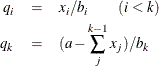
two-sided order constraints of the form:

$q_1 \le q_2 \le q_3 \le \ldots \le q_ k$

These inequality constraints can be expressed as the following set of equality constraints:

$q_1 = x_1, \quad q_2 = q_1 + x^2_2, \quad \ldots \quad q_ k = q_{k-1} + x^2_ k$

where the new parameters $x_1$ , …, $x_ k$ are unconstrained.

For example, to implement $q_1 \le q_2 \le q_3 \le q_4$ simultaneously, you can use the following statements:
```
parameters x1-x4 (4*0.);
q1 = x1;
q2 = q1 + x2 * x2;
q3 = q2 + x3 * x3;
q4 = q3 + x4 * x4;
```
In this specification, you redefine $q_1-q_4$ as dependent parameters that are functions of $x_1-x_4$ , which are defined as independent parameters in the PARAMETERS statement. Each $x_ i$ has a starting value of zero without being constrained in estimation. The order relation of $q_ i$ ’s are satisfied by the way they are computed in the SAS programming statements .
linear equation constraints of the form:

$\sum _ i^ k b_ i q_ i = a$

where $q_ i$ ’s are the parameters of interest, $b_ i$ ’s are constant coefficients, a is a constant, and k is an integer greater than one. This linear equation can be expressed as the following system of equations with unconstrained new parameters $x_1, x_2, \ldots , x_ k$ :

$\begin{eqnarray*} q_ i & = & x_ i / b_ i \qquad (i < k) \\ q_ k & = & (a - \sum _ j^{k-1} x_ j) / b_ k \end{eqnarray*}$

For example, consider the following linear constraint on independent parameters $q_1-q_3$ :

$3 q_1 + 2 q_2 - 5 q_3 = 8$

You can use the following statements to implement the linear constraint:
```
parameters x1-x2 (2*0.);
q1 = x1 / 3;
q2 = x2 / 2;
q3 = -(8 - x1 - x2) / 5;
```
In this specification, $q_1-q_3$ become dependent parameters that are functions of x1 and x2. The linear constraint on $q_1$ and $q_3$ are satisfied by the way they are computed. In addition, after reparameterization the number of independent parameters drops to two.

See McDonald (1980) and Browne (1982) for further notes on reparameterization techniques.

Explicit or Implicit Specification of Constraints?

Explicit and implicit constraint techniques differ in their specifications and lead to different computational steps in optimizing a solution. The explicit constraint specification that uses the supported statements incurs additional computational routines within the optimization steps. In contrast, the implicit reparameterization method does not incur additional routines for evaluating constraints during the optimization. Rather, it changes the constrained problem to a non-constrained one. This costs more in computing function derivatives and in storing parameters.

If the optimization problem is small enough to apply the Levenberg-Marquardt or Newton-Raphson algorithm, use the BOUNDS and the LINCON statements to set explicit boundary and linear constraints. If the problem is so large that you must use a quasi-Newton or conjugate gradient algorithm, reparameterization techniques might be more efficient than the BOUNDS and LINCON statements.

The CALIS Procedure