The MCMC Procedure
-
Overview

-
Getting Started
-
Syntax
-
Details
How PROC MCMC Works Blocking of Parameters Sampling Methods Tuning the Proposal Distribution Conjugate Sampling Initial Values of the Markov Chains Assignments of Parameters Standard Distributions Usage of Multivariate Distributions Specifying a New Distribution Using Density Functions in the Programming Statements Truncation and Censoring Some Useful SAS Functions Matrix Functions in PROC MCMC Create Design Matrix Modeling Joint Likelihood Regenerating Diagnostics Plots Caterpillar Plot Posterior Predictive Distribution Handling of Missing Data Floating Point Errors and Overflows Handling Error Messages Computational Resources Displayed Output ODS Table Names ODS Graphics
-
Examples
Simulating Samples From a Known Density Box-Cox Transformation Logistic Regression Model with a Diffuse Prior Logistic Regression Model with Jeffreys’ Prior Poisson Regression Nonlinear Poisson Regression Models Logistic Regression Random-Effects Model Nonlinear Poisson Regression Random-Effects Model Multivariate Normal Random-Effects Model Change Point Models Exponential and Weibull Survival Analysis Time Independent Cox Model Time Dependent Cox Model Piecewise Exponential Frailty Model Normal Regression with Interval Censoring Constrained Analysis Implement a New Sampling Algorithm Using a Transformation to Improve Mixing Gelman-Rubin Diagnostics
- References
Example 54.17 Implement a New Sampling Algorithm
This example illustrates using the UDS statement to implement a new Markov chain sampler. The algorithm demonstrated here is proposed by Holmes and Held (2006), hereafter referred to as HH. They presented a Gibbs sampling algorithm for generating draws from the posterior distribution of the parameters in a probit regression model. The notation follows closely to HH.
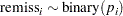
The data used here is the remission data set from a PROC LOGISTIC example:
title 'Implement a New Sampling Algorithm';
data inputdata;
   input remiss cell smear infil li blast temp;
   ind = _n_;
   cnst = 1;
   label remiss='Complete Remission';
   datalines;

   ... more lines ...

   0  1     0.73  0.73  0.7  0.398  0.986
;
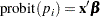
The variable remiss is the cancer remission indicator variable with a value of 1 for remission and a value of 0 for nonremission. There are six explanatory variables: cell, smear, infil, li, blast, and temp. These variables are the risk factors thought to be related to cancer remission. The binary regression model is as follows:
 |
where the covariates are linked to  through a probit transformation:
 |
 are the regression coefficients and
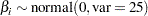
  the explanatory variables. Suppose that you want to use independent normal priors on the regression coefficients:
 |
Fitting a logistic model with PROC MCMC is straightforward. You can use the following statements:
proc mcmc data=inputdata nmc=100000 propcov=quanew seed=17
          outpost=mcmcout;
   ods select PostSummaries ess;
   parms beta0-beta6;
   prior beta: ~ normal(0,var=25);
   mu = beta0 + beta1*cell + beta2*smear +
         beta3*infil +  beta4*li + beta5*blast +  beta6*temp;
   p = cdf('normal', mu, 0, 1);
   model remiss ~ bern(p);
run;
The expression mu is the regression mean, and the CDF function links mu to the probability of remission p in the binary likelihood.
The summary statistics and effective sample sizes tables are shown in Output 54.17.1. There are high autocorrelations among the posterior samples, and efficiency is relatively low. The correlation time is reduced only after a large amount of thinning.
| Implement a New Sampling Algorithm |
| Posterior Summaries | ||||||
|---|---|---|---|---|---|---|
| Parameter | N | Mean | Standard Deviation |
Percentiles | ||
| 25% | 50% | 75% | ||||
| beta0 | 100000 | -2.0531 | 3.8299 | -4.6418 | -2.0354 | 0.5638 |
| beta1 | 100000 | 2.6300 | 2.8270 | 0.6563 | 2.5272 | 4.4846 |
| beta2 | 100000 | -0.8426 | 3.2108 | -3.0270 | -0.8263 | 1.3429 |
| beta3 | 100000 | 1.5933 | 3.5491 | -0.7993 | 1.6190 | 3.9695 |
| beta4 | 100000 | 2.0390 | 0.8796 | 1.4312 | 2.0028 | 2.6194 |
| beta5 | 100000 | -0.3184 | 0.9543 | -0.9613 | -0.3123 | 0.3418 |
| beta6 | 100000 | -3.2611 | 3.7806 | -5.8050 | -3.2736 | -0.7243 |
| Implement a New Sampling Algorithm |
| Effective Sample Sizes | |||
|---|---|---|---|
| Parameter | ESS | Autocorrelation Time |
Efficiency |
| beta0 | 4280.8 | 23.3602 | 0.0428 |
| beta1 | 4496.5 | 22.2398 | 0.0450 |
| beta2 | 3434.1 | 29.1199 | 0.0343 |
| beta3 | 3856.6 | 25.9294 | 0.0386 |
| beta4 | 3659.7 | 27.3245 | 0.0366 |
| beta5 | 3229.9 | 30.9610 | 0.0323 |
| beta6 | 4430.7 | 22.5696 | 0.0443 |
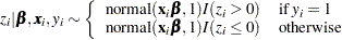
As an alternative to the random walk Metropolis, you can use the Gibbs algorithm to sample from the posterior distribution. The Gibbs algorithm is described in the section Gibbs Sampler. While the Gibbs algorithm generally applies to a wide range of statistical models, the actual implementation can be problem-specific. In this example, performing a Gibbs sampler involves introducing a class of auxiliary variables (also known as latent variables). You first reformulate the model by adding a  for each observation in the data set:
 |
 |
 |
|||
 |
|
 |
|||
 |
 |
 |
|||
 |
|
 |
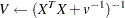
If has a normal prior, such as  , you can work out a closed form solution to the full conditional distribution of given the data and the latent variables . The full conditional distribution is also a multivariate normal, due to the conjugacy of the problem. See the section Conjugate Priors. The formula is shown here:
 |
|
 |
|||
 |
|
 |
|||
 |
|
 |
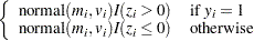
The advantage of creating the latent variables is that the full conditional distribution of  is also easy to work with. The distribution is a truncated normal distribution:
 |
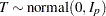
You can sample and  iteratively, by drawing given and vice verse. HH point out that a high degree of correlation could exist between and , and it makes this iterative way of sampling inefficient. As an improvement, HH proposed an algorithm that samples and jointly. At each iteration, you sample from the posterior marginal distribution (this is the distribution that is conditional only on the data and not on any parameters) and then sample from the same posterior full conditional distribution as described previously:
-
Sample
from its posterior marginal distribution: 


Sample
from the same posterior full conditional distribution described previously.
For a detailed description of each of the conditional terms, refer to the original paper.
PROC MCMC cannot sample from the probit model by using this sampling scheme but you can implement the algorithm by using the UDS statement. To sample from its marginal, you need a function that draws random variables from a truncated normal distribution. The functions, RLTNORM and RRTNORM, generate left- and right-truncated normal variates, respectively. The algorithm is taken from Robert (1995).
The functions are written in PROC FCMP (see the FCMP Procedure in the Base SAS Procedures Guide):
proc fcmp outlib=sasuser.funcs.uds;
   /******************************************/
   /* Generate left-truncated normal variate */
   /******************************************/
   function rltnorm(mu,sig,lwr);
   if lwr<mu then do;
      ans = lwr-1;
      do while(ans<lwr);
         ans = rand('normal',mu,sig);
      end;
   end;
   else do;
      mul = (lwr-mu)/sig;
      alpha = (mul + sqrt(mul**2 + 4))/2;
      accept=0;
      do while(accept=0);
         z = mul + rand('exponential')/alpha;
         lrho = -(z-alpha)**2/2;
         u = rand('uniform');
         lu = log(u);
         if lu <= lrho then accept=1;
      end;
      ans = sig*z + mu;
   end;
   return(ans);
   endsub;

   /*******************************************/
   /* Generate right-truncated normal variate */
   /*******************************************/
   function rrtnorm(mu,sig,uppr);
   ans = 2*mu - rltnorm(mu,sig, 2*mu-uppr);
   return(ans);
   endsub;
run;
The function call to RLTNORM(mu,sig,lwr) generates a random number from the left-truncated normal distribution:
 |
Similarly, the function call to RRTNORM(mu,sig,uppr) generates a random number from the right-truncated normal distribution:
 |
These functions are used to generate the latent variables .
Using the algorithm A1 from the HH paper as an example, Output 54.46 lists a line-by-line implementation with the PROC MCMC coding style. The table is broken into three portions: set up the constants, initialize the parameters, and sample one draw from the posterior distribution. The left column of the table is identical to the A1 algorithm stated in the appendix of HH. The right column of the table lists SAS statements.
Define Constants |
In the BEGINCNST/ENDCNST Statements |
||||||||||||||||||||||||||||||
|---|---|---|---|---|---|---|---|---|---|---|---|---|---|---|---|---|---|---|---|---|---|---|---|---|---|---|---|---|---|---|---|
|
|
||||||||||||||||||||||||||||||
|
call chol(v,L); |
||||||||||||||||||||||||||||||
|
call mult(v,xt,S); |
||||||||||||||||||||||||||||||
|
|
||||||||||||||||||||||||||||||
Initial Values |
In the BEGINCNST/ENDCNST Statements |
||||||||||||||||||||||||||||||
|
|
||||||||||||||||||||||||||||||
|
call mult(S,Z,B); |
||||||||||||||||||||||||||||||
Draw One Sample |
Subroutine HH |
||||||||||||||||||||||||||||||
|
|


 to
to 


The following statements define the subroutine HH (algorithm A1) in PROC FCMP and store it in library sasuser.funcs.uds:
/* define the HH algorithm in PROC FCMP. */
%let n = 27;
%let p = 7;
options cmplib=sasuser.funcs;
proc fcmp outlib=sasuser.funcs.uds;
subroutine HH(beta[*],Z[*],B[*],x[*,*],y[*],W[*],sQ[*],S[*,*],L[*,*]);
outargs beta, Z, B;
array T[&p] / nosym;
do j=1 to &n;
zold = Z[j];
m = 0;
do k = 1 to &p;
m = m + X[j,k] * B[k];
end;
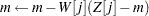
m = m - W[j]*(Z[j]-m);
if (y[j]=1) then
Z[j] = rltnorm(m,sQ[j],0);
else
Z[j] = rrtnorm(m,sQ[j],0);
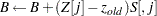
diff = Z[j] - zold;
do k = 1 to &p;
B[k] = B[k] + diff * S[k,j];
end;
end;
do j=1 to &p;
T[j] = rand('normal');
end;
call mult(L,T,T);
call addmatrix(B,T,beta);
endsub;
run;
Note that one-dimensional array arguments take the form of name[*] and two-dimensional array arguments take the form of name[*,*]. Three variables, beta, Z, and B, are OUTARGS variables, making them the only arguments that can be modified in the subroutine. For the UDS statement to work, all OUTARGS variables have to be model parameters. Technically, only beta and Z are model parameters, and B is not. The reason that B is declared as an OUTARGS is because the array must be updated throughout the simulation, and this is the only way to modify its values. The input array x contains all of the explanatory variables, and the array y stores the response. The rest of the input arrays, W, sQ, S, and L, store constants as detailed in the algorithm. The following statements illustrate how to fit a Bayesian probit model by using the HH algorithm:
options cmplib=sasuser.funcs;
proc mcmc data=inputdata nmc=5000 monitor=(beta) outpost=hhout;
ods select PostSummaries ess;
array xtx[&p,&p]; /* work space */
array xt[&p,&n]; /* work space */
array v[&p,&p]; /* work space */
array HatMat[&n,&n]; /* work space */
array S[&p,&n]; /* V * Xt */
array W[&n];
array y[1]/ nosymbols; /* y stores the response variable */
array x[1]/ nosymbols; /* x stores the explanatory variables */
array sQ[&n]; /* sqrt of the diagonal elements of Q */
array B[&p]; /* conditional mean of beta */
array L[&p,&p]; /* Cholesky decomp of conditional cov */
array Z[&n]; /* latent variables Z */
array beta[&p] beta0-beta6; /* regression coefficients */
begincnst;
call streaminit(83101);
if ind=1 then do;
rc = read_array("inputdata", x, "cnst", "cell", "smear", "infil",
"li", "blast", "temp");
rc = read_array("inputdata", y, "remiss");
call identity(v);
call mult(v, 25, v);
call transpose(x,xt);
call mult(xt,x,xtx);
call inv(v,v);
call addmatrix(xtx,v,xtx);
call inv(xtx,v);
call chol(v,L);
call mult(v,xt,S);
call mult(x,S,HatMat);
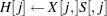
do j=1 to &n;
H = HatMat[j,j];
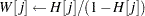
W[j] = H/(1-H);
sQ[j] = sqrt(W[j] + 1);
end;
do j=1 to &n;
if(y[j]=1) then
Z[j] = rltnorm(0,1,0);
else
Z[j] = rrtnorm(0,1,0);
end;
call mult(S,Z,B);
end;
endcnst;
uds HH(beta,Z,B,x,y,W,sQ,S,L);
parms z: beta: 0 B1-B7 / uds;
prior z: beta: B1-B7 ~ general(0);
model general(0);
run;
The OPTIONS statement names the catalog of FCMP subroutines to use. The cmplib library stores the subroutine HH. You do not need to set a random number seed in the PROC MCMC statement because all random numbers are generated from the HH subroutine. The initialization of the rand function is controlled by the streaminit function, which is called in the program with a seed value of 83101.
A number of arrays are allocated. Some of them, such as xtx, xt, v, and HatMat, allocate work space for constant arrays. Other arrays are used in the subroutine sampling. Explanations of the arrays are shown in comments in the statements.
In the BEGINCNST and ENDCNST statement block, you read data set variables in the arrays x and y, calculate all the constant terms, and assign initial values to Z and B. For the READ_ARRAY function, see the section READ_ARRAY Function. For listings of all array functions and their definitions, see the section Matrix Functions in PROC MCMC.
The UDS statement declares that the subroutine HH is used to sample the parameters beta, Z, and B. You also specify the UDS option in the PARMS statement. Because all parameters are updated through the UDS interface, it is not necessary to declare the actual form of the prior for any of the parameters. Each parameter is declared to have a prior of general(0). Similarly, it is not necessary to declare the actual form of the likelihood. The MODEL statement also takes a flat likelihood of the form general(0).
Summary statistics and effective sample sizes are shown in Output 54.17.2. The posterior estimates are very close to what was shown in Output 54.17.1. The HH algorithm produces samples that are much less correlated.
| Implement a New Sampling Algorithm |
| Posterior Summaries | ||||||
|---|---|---|---|---|---|---|
| Parameter | N | Mean | Standard Deviation |
Percentiles | ||
| 25% | 50% | 75% | ||||
| beta0 | 5000 | -2.0567 | 3.8260 | -4.6537 | -2.0777 | 0.5495 |
| beta1 | 5000 | 2.7254 | 2.8079 | 0.7812 | 2.6678 | 4.5370 |
| beta2 | 5000 | -0.8318 | 3.2017 | -2.9987 | -0.8626 | 1.2918 |
| beta3 | 5000 | 1.6319 | 3.5108 | -0.7481 | 1.6636 | 4.0302 |
| beta4 | 5000 | 2.0567 | 0.8800 | 1.4400 | 2.0266 | 2.6229 |
| beta5 | 5000 | -0.3473 | 0.9490 | -0.9737 | -0.3267 | 0.2752 |
| beta6 | 5000 | -3.3787 | 3.7991 | -5.9089 | -3.3504 | -0.7928 |
| Implement a New Sampling Algorithm |
| Effective Sample Sizes | |||
|---|---|---|---|
| Parameter | ESS | Autocorrelation Time |
Efficiency |
| beta0 | 3651.3 | 1.3694 | 0.7303 |
| beta1 | 1563.8 | 3.1973 | 0.3128 |
| beta2 | 5005.9 | 0.9988 | 1.0012 |
| beta3 | 4853.2 | 1.0302 | 0.9706 |
| beta4 | 2611.2 | 1.9148 | 0.5222 |
| beta5 | 3049.2 | 1.6398 | 0.6098 |
| beta6 | 3503.2 | 1.4273 | 0.7006 |
It is interesting to compare the two approaches of fitting a generalized linear model. The random walk Metropolis on a seven-dimensional parameter space produces autocorrelations that are substantially higher than the HH algorithm. A much longer chain is needed to produce roughly equivalent effective sample sizes. On the other hand, the Metropolis algorithm is faster to run. The running time of these two examples is roughly the same, with the random walk Metropolis with 100000 samples, a 20-fold increase over that in the HH algorithm example. The speed difference can be attributed to a number of factors, ranging from the implementation of the software and the overhead cost of calling PROC FCMP subroutine and functions. In addition, the HH algorithm requires more parameters by creating an equal number of latent variables as the sample size. Sampling more parameters takes time. A larger number of parameters also increases the challenge in convergence diagnostics, because it is imperative to have convergence in all parameters before you make valid posterior inferences. Finally, you might feel that coding in PROC MCMC is easier. However, this really is not a fair comparison to make here. Writing a Metropolis algorithm from scratch would have probably taken just as much, if not more, effort than the HH algorithm.