The MCMC Procedure
-
Overview

-
Getting Started
-
Syntax
-
Details
How PROC MCMC Works Blocking of Parameters Sampling Methods Tuning the Proposal Distribution Conjugate Sampling Initial Values of the Markov Chains Assignments of Parameters Standard Distributions Usage of Multivariate Distributions Specifying a New Distribution Using Density Functions in the Programming Statements Truncation and Censoring Some Useful SAS Functions Matrix Functions in PROC MCMC Create Design Matrix Modeling Joint Likelihood Regenerating Diagnostics Plots Caterpillar Plot Posterior Predictive Distribution Handling of Missing Data Floating Point Errors and Overflows Handling Error Messages Computational Resources Displayed Output ODS Table Names ODS Graphics
-
Examples
Simulating Samples From a Known Density Box-Cox Transformation Logistic Regression Model with a Diffuse Prior Logistic Regression Model with Jeffreys’ Prior Poisson Regression Nonlinear Poisson Regression Models Logistic Regression Random-Effects Model Nonlinear Poisson Regression Random-Effects Model Multivariate Normal Random-Effects Model Change Point Models Exponential and Weibull Survival Analysis Time Independent Cox Model Time Dependent Cox Model Piecewise Exponential Frailty Model Normal Regression with Interval Censoring Constrained Analysis Implement a New Sampling Algorithm Using a Transformation to Improve Mixing Gelman-Rubin Diagnostics
- References
Example 54.2 Box-Cox Transformation
Box-Cox transformations (Box and Cox; 1964) are often used to find a power transformation of a dependent variable to ensure the normality assumption in a linear regression model. This example illustrates how you can use PROC MCMC to estimate a Box-Cox transformation for a linear regression model. Two different priors on the transformation parameter  are considered: a continuous prior and a discrete prior. You can estimate the probability of being 0 with a discrete prior but not with a continuous prior. The IF-ELSE statements are demonstrated in the example.
Using a Continuous Prior on
The following statements create a SAS data set with measurements of y (the response variable) and x (a single dependent variable):
title 'Box-Cox Transformation, with a Continuous Prior on Lambda';
data boxcox;
   input y x @@;
   datalines;
10.0  3.0  72.6  8.3  59.7  8.1  20.1  4.8  90.1  9.8   1.1  0.9
78.2  8.5  87.4  9.0   9.5  3.4   0.1  1.4   0.1  1.1  42.5  5.1

   ... more lines ...

 2.6  1.8  58.6  7.9  81.2  8.1  37.2  6.9
 ;
The Box-Cox transformation of  takes on the form of:
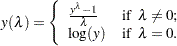 |
The transformed response  is assumed to be normally distributed:
 |
The likelihood with respect to the original response  is as follows:
 |
where  is the Jacobian:
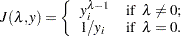 |
And on the log-scale, the Jacobian becomes:
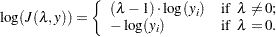 |
There are four model parameters:  and
and  . You can considering using a flat prior on
  and a gamma prior on .
To consider only power transformations ( ), you can use a continuous prior (for example, a uniform prior from
  to
to  ) on . One issue with using a continuous prior is that you cannot estimate the probability of
  . To do so, you need to consider a discrete prior that places positive probability mass on the point
  . See Modeling
  .
.
The following statements fit a Box-Cox transformation model:
ods graphics on;
proc mcmc data=boxcox nmc=50000 thin=10 propcov=quanew seed=12567
          monitor=(lda);
   ods select PostSummaries PostIntervals TADpanel;

   parms beta0 0  beta1 0  lda 1 s2 1;

   beginnodata;
   prior beta: ~ general(0);
   prior s2 ~ gamma(shape=3, scale=2);
   prior lda ~ unif(-2,2);
   sd = sqrt(s2);
   endnodata;

   ys = (y**lda-1)/lda;
   mu = beta0+beta1*x;
   ll = (lda-1)*log(y)+lpdfnorm(ys, mu, sd);
   model general(ll);
run;
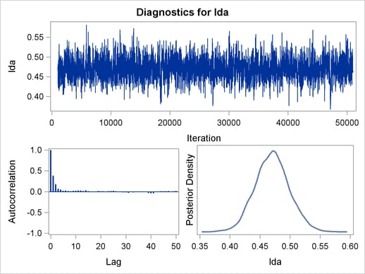
The PROPCOV= option initializes the Markov chain at the posterior mode and uses the estimated inverse Hessian matrix as the initial proposal covariance matrix. The MONITOR= option selects as the variable to report. The ODS SELECT statement displays the summary statistics table, the interval statistics table, and the diagnostic plots.
The PARMS statement puts all four parameters,  ,
,  , , and , in a single block and assigns initial values to each of them. Three PRIOR statements specify previously stated prior distributions for these parameters. The assignment to sd transforms a variance to a standard deviation. It is better to place the transformation inside the BEGINNODATA and ENDNODATA statements to save computational time.
The assignment to the symbol ys evaluates the Box-Cox transformation of y, where mu is the regression mean and ll is the log likelihood of the transformed variable ys. Note that the log of the Jacobian term is included in the calculation of ll.
Summary statistics and interval statistics for lda are listed in Output 54.2.1.
| Box-Cox Transformation, with a Continuous Prior on Lambda |
| Posterior Summaries | ||||||
|---|---|---|---|---|---|---|
| Parameter | N | Mean | Standard Deviation |
Percentiles | ||
| 25% | 50% | 75% | ||||
| lda | 5000 | 0.4702 | 0.0284 | 0.4515 | 0.4703 | 0.4884 |
| Posterior Intervals | |||||
|---|---|---|---|---|---|
| Parameter | Alpha | Equal-Tail Interval | HPD Interval | ||
| lda | 0.050 | 0.4162 | 0.5269 | 0.4197 | 0.5298 |
The posterior mean of is  , with a
  equal-tail interval of
  and a similar HPD interval. The prefered power transformation would be
  (rounding up to the square root transformation).
Output 54.2.2 shows diagnostics plots for lda. The chain appears to converge, and you can proceed to make inferences. The density plot shows that the posterior density is relatively symmetric around its mean estimate.
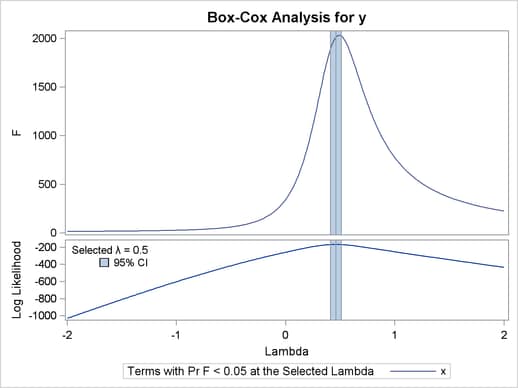
To verify the results, you can use PROC TRANSREG (see
Chapter 93,
The TRANSREG Procedure
) to find the estimate of .
proc transreg data=boxcox details pbo;
   ods output boxcox = bc;
   model boxcox(y / convenient lambda=-2 to 2 by 0.01) = identity(x);
   output out=trans;
run;
Output from PROC TRANSREG is shown in Output 54.2.5 and Output 54.2.4. PROC TRANSREG produces a similar point estimate of  , and the 95% confidence interval is shown in Output 54.2.5.
| Box-Cox Transformation, with a Continuous Prior on Lambda |
| Model Statement Specification Details | ||||
|---|---|---|---|---|
| Type | DF | Variable | Description | Value |
| Dep | 1 | BoxCox(y) | Lambda Used | 0.5 |
| Lambda | 0.46 | |||
| Log Likelihood | -167.0 | |||
| Conv. Lambda | 0.5 | |||
| Conv. Lambda LL | -168.3 | |||
| CI Limit | -169.0 | |||
| Alpha | 0.05 | |||
| Options | Convenient Lambda Used | |||
| Ind | 1 | Identity(x) | DF | 1 |
The ODS data set Bc contains the 95% confidence interval estimates produced by PROC TRANSREG. This ODS table is rather large, and you want to see only the relevant portion. The following statements generate the part of the table that is important and display Output 54.2.5:
proc print noobs label data=bc(drop=rmse);
   title2 'Confidence Interval';
   where ci ne ' ' or abs(lambda - round(lambda, 0.5)) < 1e-6;
   label convenient = '00'x ci = '00'x;
run;
The estimated 90% confidence interval is  , which is very close to the reported Bayesian credible intervals. The resemblance of the intervals is probably due to the noninformative prior that you used in this analysis.
| Box-Cox Transformation, with a Continuous Prior on Lambda |
| Confidence Interval |
| Dependent | Lambda | R-Square | Log Likelihood | ||
|---|---|---|---|---|---|
| BoxCox(y) | -2.00 | 0.14 | -1030.56 | ||
| BoxCox(y) | -1.50 | 0.17 | -810.50 | ||
| BoxCox(y) | -1.00 | 0.22 | -602.53 | ||
| BoxCox(y) | -0.50 | 0.39 | -415.56 | ||
| BoxCox(y) | 0.00 | 0.78 | -257.92 | ||
| BoxCox(y) | 0.41 | 0.95 | -168.40 | * | |
| BoxCox(y) | 0.42 | 0.95 | -167.86 | * | |
| BoxCox(y) | 0.43 | 0.95 | -167.46 | * | |
| BoxCox(y) | 0.44 | 0.95 | -167.19 | * | |
| BoxCox(y) | 0.45 | 0.95 | -167.05 | * | |
| BoxCox(y) | 0.46 | 0.95 | -167.04 | < | |
| BoxCox(y) | 0.47 | 0.95 | -167.16 | * | |
| BoxCox(y) | 0.48 | 0.95 | -167.41 | * | |
| BoxCox(y) | 0.49 | 0.95 | -167.79 | * | |
| BoxCox(y) | 0.50 | + | 0.95 | -168.28 | * |
| BoxCox(y) | 0.51 | 0.95 | -168.89 | * | |
| BoxCox(y) | 1.00 | 0.89 | -253.09 | ||
| BoxCox(y) | 1.50 | 0.79 | -345.35 | ||
| BoxCox(y) | 2.00 | 0.70 | -435.01 |
Modeling
With a continuous prior on , you can get only a continuous posterior distribution, and this makes the probability of  equal to by definition. To consider as a viable solution to the Box-Cox transformation, you need to use a discrete prior that places some probability mass on the point 0 and allows for a meaningful posterior estimate of .
This example uses a simulation study where the data are generated from an exponential likelihood. The simulation implies that the correct transformation should be the logarithm and should be 0. Consider the following exponential model:
 |
where  . The transformed data can be fitted with a linear model:
 |
The following statements generate a SAS data set with a gridded x and corresponding y:
title 'Box-Cox Transformation, Modeling Lambda = 0';
data boxcox;
   do x = 1 to 8 by 0.025;
      ly = x + normal(7);
      y = exp(ly);
      output;
   end;
run;
The log-likelihood function, after taking the Jacobian into consideration, is as follows:
 |
where  and
and  are two constants.
You can use the function DGENERAL to place a discrete prior on . The function is similar to the function GENERAL, except that it indicates a discrete distribution. For example, you can specify a discrete uniform prior from to using
prior lda ~ dgeneral(1, lower=-2, upper=2);
This places equal probability mass on five points, ,  , ,
, ,  , and . This prior might not work well here because the grid is too coarse. To consider smaller values of , you can sample a parameter that takes a wider range of integer values and transform it back to the space. For example, set alpha as your model parameter and give it a discrete uniform prior from
  to
to  . Then define as alpha/100 so can take values between and but on a finer grid.
The following statements fit a Box-Cox transformation by using a discrete prior on :
proc mcmc data=boxcox outpost=simout nmc=50000 thin=10 seed=12567
          monitor=(lda);

   ods select PostSummaries PostIntervals;
   parms s2 1 alpha 10;

   beginnodata;
   prior s2 ~ gamma(shape=3, scale=2);
   if alpha=0 then lp = log(2);
      else lp = log(1);
   prior alpha ~ dgeneral(lp, lower=-200, upper=200);
   lda = alpha * 0.01;
   sd = sqrt(s2);
   endnodata;

   if alpha=0 then
      ll = -ly+lpdfnorm(ly, x, sd);
   else do;
      ys = (y**lda - 1)/lda;
      ll = (lda-1)*ly+lpdfnorm(ys, x, sd);
   end;
   model general(ll);
run;
There are two parameters, s2 and alpha, in the model. They are placed in a single PARMS statement so that they are sampled in the same block.
The parameter s2 takes a gamma distribution, and alpha takes a discrete prior. The IF-ELSE statements state that alpha takes twice as much prior density when it is 0 than otherwise. Note that on the original scale,  . Translating that to the log scale, the densities become
  and
and  , respectively. The lda assignment statement transforms alpha to the parameter of interest: lda takes values between and . You can model lda on a even smaller scale by dividing alpha by a larger constant. However, an increment of 0.01 in the Box-Cox transformation is usually sufficient. The sd assignment statement calculates the square root of the variance term.
The log-likelihood function uses another set of IF-ELSE statements, separating the case of from the others. The formulas are stated previously. The output of the program is shown in Output 54.2.6.
| Box-Cox Transformation, Modeling Lambda = 0 |
| Posterior Summaries | ||||||
|---|---|---|---|---|---|---|
| Parameter | N | Mean | Standard Deviation |
Percentiles | ||
| 25% | 50% | 75% | ||||
| lda | 5000 | -0.00002 | 0.00201 | 0 | 0 | 0 |
| Posterior Intervals | |||||
|---|---|---|---|---|---|
| Parameter | Alpha | Equal-Tail Interval | HPD Interval | ||
| lda | 0.050 | 0 | 0 | 0 | 0 |
From the summary statistics table, you see that the point estimate for is 0 and both of the 95% equal-tail and HPD credible intervals are 0. This strongly suggests that is the best estimate for this problem. In addition, you can also count the frequency of among posterior samples to get a more precise estimate on the posterior probability of being 0.
The following statements use PROC FREQ to produce Output 54.2.7 and Output 54.2.8:
proc freq data=simout;
   ods select onewayfreqs freqplot;
   tables lda /nocum plot=freqplot(scale=percent);
run;
ods graphics off;
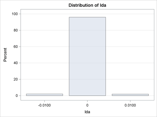
Output 54.2.7 shows the frequency count table. An estimate of  is
is  . The conclusion is that the
  transformation should be the appropriate transformation used here, which agrees with the simulation setup. Output 54.2.8 shows the histogram of .
| Box-Cox Transformation, Modeling Lambda = 0 |
| lda | Frequency | Percent |
|---|---|---|
| -0.0100 | 106 | 2.12 |
| 0 | 4798 | 95.96 |
| 0.0100 | 96 | 1.92 |