The MCMC Procedure
-
Overview

-
Getting Started
-
Syntax
-
Details
How PROC MCMC Works Blocking of Parameters Sampling Methods Tuning the Proposal Distribution Conjugate Sampling Initial Values of the Markov Chains Assignments of Parameters Standard Distributions Usage of Multivariate Distributions Specifying a New Distribution Using Density Functions in the Programming Statements Truncation and Censoring Some Useful SAS Functions Matrix Functions in PROC MCMC Create Design Matrix Modeling Joint Likelihood Regenerating Diagnostics Plots Caterpillar Plot Posterior Predictive Distribution Handling of Missing Data Floating Point Errors and Overflows Handling Error Messages Computational Resources Displayed Output ODS Table Names ODS Graphics
-
Examples
Simulating Samples From a Known Density Box-Cox Transformation Logistic Regression Model with a Diffuse Prior Logistic Regression Model with Jeffreys’ Prior Poisson Regression Nonlinear Poisson Regression Models Logistic Regression Random-Effects Model Nonlinear Poisson Regression Random-Effects Model Multivariate Normal Random-Effects Model Change Point Models Exponential and Weibull Survival Analysis Time Independent Cox Model Time Dependent Cox Model Piecewise Exponential Frailty Model Normal Regression with Interval Censoring Constrained Analysis Implement a New Sampling Algorithm Using a Transformation to Improve Mixing Gelman-Rubin Diagnostics
- References
Example 54.12 Time Independent Cox Model
This example has two purposes. One is to illustrate how to use PROC MCMC to fit a Cox proportional hazard model. Specifically, the time independent model. See Time Dependent Cox Model for an example on fitting time dependent Cox model. Note that it is much easier to fit a Bayesian Cox model by specifying the BAYES statement in PROC PHREG (see Chapter 66, The PHREG Procedure ). If you are interested only in fitting a Cox regression survival model, you should use PROC PHREG.
The second objective of this example is to demonstrate how to model data that are not independent. That is the case where the likelihood for observation  depends on other observations in the data set. In other words, if you work with a likelihood function that cannot be broken down simply as
  , you can use this example for illustrative purposes. By default, PROC MCMC assumes that the programming statements and model specification is intended for a single row of observations in the data set. The Cox model is chosen because the complexity in the data structure requires more elaborate coding.
The Cox proportional hazard model is widely used in the analysis of survival time, failure time, or other duration data to explain the effect of exogenous explanatory variables. The data set used in this example is taken from Krall, Uthoff, and Harley (1975), who analyzed data from a study on myeloma in which researchers treated 65 patients with alkylating agents. Of those patients, 48 died during the study and 17 survived. The following statements generate the data set that is used in this example:
data Myeloma;
   input Time Vstatus LogBUN HGB Platelet Age LogWBC Frac
         LogPBM Protein SCalc;
   label Time='survival time'
         VStatus='0=alive 1=dead';
   datalines;
 1.25  1  2.2175   9.4  1  67  3.6628  1  1.9542  12  10
 1.25  1  1.9395  12.0  1  38  3.9868  1  1.9542  20  18
 2.00  1  1.5185   9.8  1  81  3.8751  1  2.0000   2  15

   ... more lines ...

77.00  0  1.0792  14.0  1  60  3.6812  0  0.9542   0  12
;
proc sort data = Myeloma;
   by descending time;
run;

data _null_;
   set Myeloma nobs=_n;
   call symputx('N', _n);
   stop;
run;
The variable Time represents the survival time in months from diagnosis. The variable VStatus consists of two values, 0 and 1, indicating whether the patient was alive or dead, respectively, at the end of the study. If the value of VStatus is 0, the corresponding value of Time is censored. The variables thought to be related to survival are LogBUN ( at diagnosis), HGB (hemoglobin at diagnosis), Platelet (platelets at diagnosis: 0=abnormal, 1=normal), Age (age at diagnosis in years), LogWBC (log(WBC) at diagnosis), Frac (fractures at diagnosis: 0=none, 1=present), LogPBM (log percentage of plasma cells in bone marrow), Protein (proteinuria at diagnosis), and SCalc (serum calcium at diagnosis). Interest lies in identifying important prognostic factors from these explanatory variables. In addition, there are 65 (&n) observations in the data set Myeloma. The likelihood used in these examples is the Brewslow likelihood:
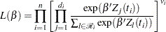 |
where
 is the vector parameters
  is the total number of observations in the data set
  is the th time, which can be either event time or censored time
  is the vector explanatory variables for the
  th individual at time
 is the multiplicity of failures at . If there are no ties in time, is 1 for all .
  is the risk set for the th time , which includes all observations that have survival time greater than or equal to
  indicates whether the patient is censored. The value 0 corresponds to censoring. Note that the censored time enters the likelihood function only through the formation of the risk set .
Priors on the coefficients are independent normal priors with very large variance (1e6). Throughout this example, the symbol bZ represents the regression term  in the likelihood, and the symbol S represents the term
 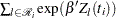 .
.
The regression model considered in this example uses the following formula:
 |
 |
 |
|||
 |
|
 |
The hard part of coding this in PROC MCMC is the construction of the risk set . contains all observations that have survival time greater than or equal to . First suppose that there are no ties in time. Sorting the data set by the variable time into descending order gives you that is in the right order. Observation ’s risk set consists of all data points  such that
  in the data set. You can cumulatively increment S in the SAS statements.
With potential ties in time, at observation , you need to know whether any subsequent observations,  and so on, have the same survival time as . Suppose that the th, the th, and the
  th observations all have the same survival time; all three of them need to be included in the risk set calculation. This means that to calculate the likelihood for some observations, you need to access both the previous and subsequent observations in the data set. There are two ways to do this. One is to use the LAG function; the other is to use the option JOINTMODEL.
The LAG function returns values from a queue (see SAS Language Reference: Dictionary). So for the th observation, you can use LAG1 to access variables from the previous row in the data set. You want to compare the lag1 value of time with the current time value. Depending on whether the two time values are equal, you can add correction terms in the calculation for the risk set S.
The following statements sort the data set by time into descending order, with the largest survival time on top:
title 'Cox Model with Time Independent Covariates';
proc freq data=myeloma;
   ods select none;
   tables time / out=freqs;
run;

proc sort data = freqs;
   by descending time;
run;

data myelomaM;
   set myeloma;
   ind = _N_;
run;
ods select all;
The following statements run PROC MCMC and produce Output 54.12.1:
proc mcmc data=myelomaM outpost=outi nmc=50000 ntu=3000 seed=1;
   ods select PostSummaries PostIntervals;
   array beta[9];
   parms beta: 0;
   prior beta: ~ normal(0, var=1e6);

   bZ = beta1 * LogBUN + beta2 * HGB + beta3 * Platelet
      + beta4 * Age + beta5 * LogWBC + beta6 * Frac +
      beta7 * LogPBM + beta8 * Protein + beta9 * SCalc;

   if ind = 1 then do;        /* first observation         */
      S = exp(bZ);
      l = vstatus * bZ;
      v = vstatus;
   end;
   else if (1 < ind < &N) then do;
      if (lag1(time) ne time) then do;
         l = vstatus * bZ;
         l = l - v * log(S);  /* correct the loglike value   */
         v = vstatus;         /* reset v count value         */
         S = S + exp(bZ);
      end;
      else do;                /* still a tie                 */
         l = vstatus * bZ;
         S = S + exp(bZ);
         v = v + vstatus;     /* add # of nonsensored values */
      end;
   end;
   else do;                   /* last observation            */
      if (lag1(time) ne time) then do;
         l = - v * log(S);    /* correct the loglike value   */
         S = S + exp(bZ);
         l = l + vstatus * (bZ - log(S));
      end;
      else do;
         S = S + exp(bZ);
         l = vstatus * bZ - (v + vstatus) * log(S);
      end;
   end;
   model general(l);
run;
The symbol bZ is the regression term, which is independent of the time variable. The symbol ind indexes observation numbers in the data set. The symbol S keeps track of the risk set term for every observation. The symbol l calculates the log likelihood for each observation. Note that the value of l for observation ind is not necessarily the correct log likelihood value for that observation, especially in cases where the observation ind is in the tied times. Correction terms are added to subsequent values of l when the time variable becomes different in order to make up the difference. The total sum of l calculated over the entire data set is correct. The symbol v keeps track of the sum of vstatus, as censored data do not enter the likelihood and need to be taken out.
You use the function LAG1 to detect if two adjacent time values are different. If they are, you know that the current observation is in a different risk set than the last one. You then need to add a correction term to the log likelihood value of l. The IF-ELSE statements break the observations into three parts: the first observation, the last observation and everything in the middle.
| Cox Model with Time Independent Covariates |
| Posterior Summaries | ||||||
|---|---|---|---|---|---|---|
| Parameter | N | Mean | Standard Deviation |
Percentiles | ||
| 25% | 50% | 75% | ||||
| beta1 | 50000 | 1.7600 | 0.6441 | 1.3275 | 1.7651 | 2.1947 |
| beta2 | 50000 | -0.1308 | 0.0720 | -0.1799 | -0.1304 | -0.0817 |
| beta3 | 50000 | -0.2017 | 0.5148 | -0.5505 | -0.1965 | 0.1351 |
| beta4 | 50000 | -0.0126 | 0.0194 | -0.0257 | -0.0128 | 0.000641 |
| beta5 | 50000 | 0.3373 | 0.7256 | -0.1318 | 0.3505 | 0.8236 |
| beta6 | 50000 | 0.3992 | 0.4337 | 0.0973 | 0.3864 | 0.6804 |
| beta7 | 50000 | 0.3749 | 0.4861 | 0.0464 | 0.3636 | 0.6989 |
| beta8 | 50000 | 0.0106 | 0.0271 | -0.00723 | 0.0118 | 0.0293 |
| beta9 | 50000 | 0.1272 | 0.1064 | 0.0579 | 0.1300 | 0.1997 |
| Posterior Intervals | |||||
|---|---|---|---|---|---|
| Parameter | Alpha | Equal-Tail Interval | HPD Interval | ||
| beta1 | 0.050 | 0.4649 | 3.0214 | 0.5117 | 3.0465 |
| beta2 | 0.050 | -0.2704 | 0.0114 | -0.2746 | 0.00524 |
| beta3 | 0.050 | -1.2180 | 0.8449 | -1.2394 | 0.7984 |
| beta4 | 0.050 | -0.0501 | 0.0257 | -0.0512 | 0.0245 |
| beta5 | 0.050 | -1.1233 | 1.7232 | -1.1124 | 1.7291 |
| beta6 | 0.050 | -0.4136 | 1.2970 | -0.4385 | 1.2575 |
| beta7 | 0.050 | -0.5551 | 1.3593 | -0.5423 | 1.3689 |
| beta8 | 0.050 | -0.0451 | 0.0618 | -0.0451 | 0.0616 |
| beta9 | 0.050 | -0.0933 | 0.3272 | -0.0763 | 0.3406 |
An alternative to using the LAG function is to use the PROC option JOINTMODEL. With this option, the log-likelihood function you specify applies not to a single observation but to the entire data set. See Modeling Joint Likelihood for details on how to properly use this option. The basic idea is that you store all necessary data set variables in arrays and use only the arrays to construct the log likelihood of the entire data set. This approach works here because for every observation , you can use index to access different values of arrays to construct the risk set S. To use the JOINTMODEL option, you need to do some additional data manipulation. You want to create a stop variable for each observation, which indicates the observation number that should be included in S for that observation. For example, if observations 4, 5, 6 all have the same survival time, the stop value for all of them is 6.
The following statements generate a new data set MyelomaM that contains the stop variable:
data myelomaM;
   merge myelomaM freqs(drop=percent);
   by descending time;
   retain stop;
   if first.time then do;
      stop = _n_ + count - 1;
   end;
run;
The following SAS program fits the same Cox model by using the JOINTMODEL option:
data a;
   run;

proc mcmc data=a outpost=outa nmc=50000 ntu=3000 seed=1 jointmodel;
   ods select none;
      array beta[9];
      array data[1] / nosymbols;
      array timeA[1] / nosymbols;
      array vstatusA[1] / nosymbols;
      array stopA[1] / nosymbols;
      array bZ[&n];
      array S[&n];

      begincnst;
      rc = read_array("myelomam", data, "logbun", "hgb", "platelet",
                      "age", "logwbc", "frac", "logpbm", "protein", "scalc");
      rc = read_array("myelomam", timeA, "time");
      rc = read_array("myelomam", vstatusA, "vstatus");
      rc = read_array("myelomam", stopA, "stop");
      endcnst;

      parms (beta:) 0;
      prior beta: ~ normal(0, var=1e6);

      jl = 0;
      /* calculate each bZ and cumulatively adding S as if there are no ties.*/
      call mult(data, beta, bZ);
      S[1] = exp(bZ[1]);
      do i = 2 to &n;
         S[i] = S[i-1] + exp(bZ[i]);
      end;

      do i = 1 to &n;
         /* correct the S[i] term, when needed. */
         if(stopA[i] > i) then do;
            do j = (i+1) to stopA[i];
               S[i] = S[i] + exp(bZ[j]);
            end;
         end;
         jl = jl + vstatusA[i] * (bZ[i] - log(S[i]));
      end;
      model general(jl);
run;
ods select all;
No output tables were produced because this PROC MCMC run produces identical posterior samples as does the previous example.
Because the JOINTMODEL option is specified here, you do not need to specify myelomaM as the input data set. An empty data set a is used to speed up the procedure run.
Multiple ARRAY statements allocate array symbols that are used to store the parameters (beta), the response and the covariates (data, timeA, vstatusA, and stopA), and the work space (bZ and S). The data, timeA, vstatusA, and stopA arrays are declared with the /NOSYMBOLS option. This option enables PROC MCMC to dynamically resize these arrays to match the dimensions of the input data set. See the section READ_ARRAY Function. The bZ and S arrays store the regression term and the risk set term for every observation.
The BEGINCNST and ENDCNST statements enclose programming statements that read the data set variables into these arrays. The rest of the programming statements construct the log likelihood for the entire data set.
The CALL MULT function calculates the regression term in the model and stores the result in the array bZ. In the first DO loop, you sum the risk set term S as if there are no ties in time. This underevaluates some of the S elements. For observations that have a tied time, you make the necessary correction to the corresponding S values. The correction takes place in the second DO loop. Any observation that has a tied time also has a stopA[i] that is different from i. You add the right terms to S and sum up the joint log likelihood jl. The MODEL statement specifies that the log likelihood takes on the value of jl.
To see that you get identical results from these two approaches, use PROC COMPARE to compare the posterior samples from two runs:
proc compare data=outi compare=outa;
   ods select comparesummary;
   var beta1-beta9;
run;
The output is not shown here.
Generally, the JOINTMODEL option can be slightly faster than using the default setup. The savings come from avoiding the overhead cost of accessing the data set repeatedly at every iteration. However, the speed gain is not guaranteed because it largely depends on the efficiency of your programs.
PROC PHREG fits the same model, and you get very similar results to PROC MCMC. The following statements fit the model using PROC PHREG and produce Output 54.12.2:
proc phreg data=Myeloma;
   ods select PostSummaries PostIntervals;
   model Time*VStatus(0)=LogBUN HGB Platelet Age LogWBC
                         Frac LogPBM Protein Scalc;
   bayes seed=1 nmc=10000 outpost=phout;
run;
| Cox Model with Time Independent Covariates |
| Posterior Summaries | ||||||
|---|---|---|---|---|---|---|
| Parameter | N | Mean | Standard Deviation |
Percentiles | ||
| 25% | 50% | 75% | ||||
| LogBUN | 10000 | 1.7610 | 0.6593 | 1.3173 | 1.7686 | 2.2109 |
| HGB | 10000 | -0.1279 | 0.0727 | -0.1767 | -0.1287 | -0.0789 |
| Platelet | 10000 | -0.2179 | 0.5169 | -0.5659 | -0.2360 | 0.1272 |
| Age | 10000 | -0.0130 | 0.0199 | -0.0264 | -0.0131 | 0.000492 |
| LogWBC | 10000 | 0.3150 | 0.7451 | -0.1718 | 0.3321 | 0.8253 |
| Frac | 10000 | 0.3766 | 0.4152 | 0.0881 | 0.3615 | 0.6471 |
| LogPBM | 10000 | 0.3792 | 0.4909 | 0.0405 | 0.3766 | 0.7023 |
| Protein | 10000 | 0.0102 | 0.0267 | -0.00745 | 0.0106 | 0.0283 |
| SCalc | 10000 | 0.1248 | 0.1062 | 0.0545 | 0.1273 | 0.1985 |
| Posterior Intervals | |||||
|---|---|---|---|---|---|
| Parameter | Alpha | Equal-Tail Interval | HPD Interval | ||
| LogBUN | 0.050 | 0.4418 | 3.0477 | 0.4107 | 2.9958 |
| HGB | 0.050 | -0.2718 | 0.0150 | -0.2801 | 0.00599 |
| Platelet | 0.050 | -1.1952 | 0.8296 | -1.1871 | 0.8341 |
| Age | 0.050 | -0.0514 | 0.0259 | -0.0519 | 0.0251 |
| LogWBC | 0.050 | -1.2058 | 1.7228 | -1.1783 | 1.7483 |
| Frac | 0.050 | -0.3995 | 1.2316 | -0.4273 | 1.2021 |
| LogPBM | 0.050 | -0.5652 | 1.3671 | -0.5939 | 1.3241 |
| Protein | 0.050 | -0.0437 | 0.0611 | -0.0405 | 0.0637 |
| SCalc | 0.050 | -0.0935 | 0.3264 | -0.0846 | 0.3322 |