The MCMC Procedure
-
Overview

-
Getting Started
-
Syntax
-
Details
How PROC MCMC Works Blocking of Parameters Sampling Methods Tuning the Proposal Distribution Conjugate Sampling Initial Values of the Markov Chains Assignments of Parameters Standard Distributions Usage of Multivariate Distributions Specifying a New Distribution Using Density Functions in the Programming Statements Truncation and Censoring Some Useful SAS Functions Matrix Functions in PROC MCMC Create Design Matrix Modeling Joint Likelihood Regenerating Diagnostics Plots Caterpillar Plot Posterior Predictive Distribution Handling of Missing Data Floating Point Errors and Overflows Handling Error Messages Computational Resources Displayed Output ODS Table Names ODS Graphics
-
Examples
Simulating Samples From a Known Density Box-Cox Transformation Logistic Regression Model with a Diffuse Prior Logistic Regression Model with Jeffreys’ Prior Poisson Regression Nonlinear Poisson Regression Models Logistic Regression Random-Effects Model Nonlinear Poisson Regression Random-Effects Model Multivariate Normal Random-Effects Model Change Point Models Exponential and Weibull Survival Analysis Time Independent Cox Model Time Dependent Cox Model Piecewise Exponential Frailty Model Normal Regression with Interval Censoring Constrained Analysis Implement a New Sampling Algorithm Using a Transformation to Improve Mixing Gelman-Rubin Diagnostics
- References
Example 54.16 Constrained Analysis
Conjoint analysis uses regression techniques to model consumer preferences and to estimate consumer utility functions. A problem with conventional conjoint analysis is that sometimes your estimated utilities do not make sense. Your results might suggest, for example, that the consumers would prefer to spend more on a product than to spend less. With PROC MCMC, you can specify constraints on the part-worth utilities (parameter estimates). Suppose that the consumer product being analyzed is an off-road motorcycle. The relevant attributes are how large each motorcycle is (less than 300cc, 301–550cc, and more than 551cc), how much it costs (less than $5000, $5001–$6000, $6001–$7000, and more than $7000), whether or not it has an electric starter, whether or not the engine is counter-balanced, and whether the bike is from Japan or Europe. The preference variable is a ranking of the bikes. You could perform an ordinary conjoint analysis with PROC TRANSREG (see Chapter 93, The TRANSREG Procedure ) as follows:
options validvarname=any;
proc format;
   value sizef  1 = '< 300cc' 2 = '300-550cc' 3 = '> 551cc';
   value pricef 1 = '< $5000' 2 = '$5000 - $6000'
                3 = '$6001 - $7000' 4 = '> $7000';
   value startf 1 = 'Electric Start' 2 = 'Kick Start';
   value balf   1 = 'Counter Balanced' 2 = 'Unbalanced';
   value orif   1 = 'Japanese' 2 = 'European';
run;
data bikes;
   input Size Price Start Balance Origin Rank @@;
   format size sizef. price pricef. start startf.
          balance balf. origin orif.;
   datalines;
2 1 2 1 2  3  1 4 2 2 2  7  1 2 1 1 2  6
3 3 1 1 2  1  1 3 2 1 1  5  3 4 2 2 2 12
2 3 2 2 1  9  1 1 1 2 1  8  2 2 1 2 2 10
2 4 1 1 1  4  3 1 1 2 1 11  3 2 2 1 1  2
;
title 'Ordinary Conjoint Analysis by PROC TRANSREG';
proc transreg data=bikes utilities cprefix=0 lprefix=0;
   ods select Utilities;
   model identity(rank / reflect) =
         class(size price start balance origin / zero=sum);
   output out=coded(drop=intercept) replace;
run;
The DATA step reads the experimental design and dependent variable Rank and assigns formats to label the factor levels. PROC TRANSREG is run specifying UTILITIES, which requests a conjoint analysis. The rank variable is reflected around its mean (1  12, 2 11, ..., 12 1) so that in the analysis, larger part-worth utilities correspond to higher preference. The OUT=CODED data set contains the reflected ranks and a binary coding of the factors that can be used in other analyses. Refer to Kuhfeld (2004) for more information about conjoint analysis and coding with PROC TRANSREG.
The Utilities table from the conjoint analysis is shown in Output 54.16.1. Notice the part-worth utilities for price. The part-worth utility for < $5000 is 0.25. As price increases to the $5000–$6000 range, utility decreases to  . Then as price increases to the $6001–$7000 range, part-worth utility increases to 0.5. Finally, for the most expensive bikes, utility decreases again to
  . In cases like this, you might want to impose constraints on the solution so that the part-worth utility for price never increases as prices go up.
| Ordinary Conjoint Analysis by PROC TRANSREG |
| Utilities Table Based on the Usual Degrees of Freedom | ||||
|---|---|---|---|---|
| Label | Utility | Standard Error | Importance (% Utility Range) |
Variable |
| Intercept | 6.5000 | 0.95743 | Intercept | |
| < 300cc | -0.0000 | 1.35401 | 0.000 | Class.< 300cc |
| 300-550cc | -0.0000 | 1.35401 | Class.300-550cc | |
| > 551cc | 0.0000 | 1.35401 | Class.> 551cc | |
| < $5000 | 0.2500 | 1.75891 | 13.333 | Class.< $5000 |
| $5000 - $6000 | -0.5000 | 1.75891 | Class.$5000 - $6000 | |
| $6001 - $7000 | 0.5000 | 1.75891 | Class.$6001 - $7000 | |
| > $7000 | -0.2500 | 1.75891 | Class.> $7000 | |
| Electric Start | -0.1250 | 1.01550 | 3.333 | Class.Electric Start |
| Kick Start | 0.1250 | 1.01550 | Class.Kick Start | |
| Counter Balanced | 3.0000 | 1.01550 | 80.000 | Class.Counter Balanced |
| Unbalanced | -3.0000 | 1.01550 | Class.Unbalanced | |
| Japanese | -0.1250 | 1.01550 | 3.333 | Class.Japanese |
| European | 0.1250 | 1.01550 | Class.European | |
You could run PROC TRANSREG again, specifying monotonicity constraints on the part-worth utilities for price:
title 'Constrained Conjoint Analysis by PROC TRANSREG';
proc transreg data=bikes utilities cprefix=0 lprefix=0;
   ods select ConservUtilities;
   model identity(rank / reflect) =
         monotone(price / tstandard=center)
         class(size start balance origin / zero=sum);
run;
The output from this PROC TRANSREG step is shown in Output 54.16.2.
| Constrained Conjoint Analysis by PROC TRANSREG |
| Utilities Table Based on Conservative Degrees of Freedom | ||||
|---|---|---|---|---|
| Label | Utility | Standard Error | Importance (% Utility Range) |
Variable |
| Intercept | 6.5000 | 0.97658 | Intercept | |
| Price | -0.1581 | . | 7.143 | Monotone(Price) |
| < $5000 | 0.2500 | . | ||
| $5000 - $6000 | 0.0000 | . | ||
| $6001 - $7000 | 0.0000 | . | ||
| > $7000 | -0.2500 | . | ||
| < 300cc | -0.0000 | 1.38109 | 0.000 | Class.< 300cc |
| 300-550cc | 0.0000 | 1.38109 | Class.300-550cc | |
| > 551cc | 0.0000 | 1.38109 | Class.> 551cc | |
| Electric Start | -0.2083 | 1.00663 | 5.952 | Class.Electric Start |
| Kick Start | 0.2083 | 1.00663 | Class.Kick Start | |
| Counter Balanced | 3.0000 | 0.97658 | 85.714 | Class.Counter Balanced |
| Unbalanced | -3.0000 | 0.97658 | Class.Unbalanced | |
| Japanese | -0.0417 | 1.00663 | 1.190 | Class.Japanese |
| European | 0.0417 | 1.00663 | Class.European | |
This monotonicity constraint is one of the few constraints on the part-worth utilities that you can specify in PROC TRANSREG. In contrast, PROC MCMC enables you to specify any constraint that can be written in the DATA step language. You can perform the restricted conjoint analysis with PROC MCMC by using the coded factors that were output from PROC TRANSREG. The data set is Coded.
The likelihood is a simple regression model:
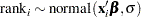 |
where rank is the response, the covariates are ‘< 300cc’n, ‘300-500cc’n, ‘< $5000’n, ‘$5000 - $6000’n, ‘$6001 - $7000’n, ‘Electric Start’n, ‘Counter Balanced’n, and Japanese. Note that OPTIONS VALIDVARNAME=ANY enables PROC TRANSREG to create names for the coded variables with blanks and special characters. That is why the name-literal notation (‘variable-name’n) is used for the input data set variables.
Suppose that there are two constraints you want to put on some of the parameters: one is that the parameters for ‘< $5000’n, ‘$5000 - $6000’n, and ‘$6001 - $7000’n decrease in order, and the other is that the parameter for ‘Counter Balanced’n is strictly positive. You can consider a truncated multivariate normal prior as follows:
 |
with the following set of constraints:
 |
 |
 |
|||
 |
|
 |
The condition that 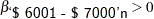 reflects an implied constraint that, by definition,
  is the utility for the highest price range, > $7000, which is the reference level for the binary coded price variable. The following statements fit the desired model:
title 'Bayesian Constrained Conjoint Analysis by PROC MCMC';
proc mcmc data=coded outpost=bikesout ntu=3000 nmc=50000 thin=10
          seed=448;
   ods select PostSummaries;
   array sigma[4,4] sigma1-sigma16;
   array mu[4] mu1-mu4;

   begincnst;
      call identity(sigma);
      call mult(sigma, 100, sigma);
      call zeromatrix(mu);
      rc = logmpdfsetsq('v', of sigma1-sigma16);
   endcnst;

   parms intercept pw300cc pw300_550cc pwElectricStart pwJapanese ltau 1;
   parms pw5000 0.3 pw5000_6000 0.2 pw6001_7000 0.1 pwCounterBalanced 1;

   beginnodata;
   prior intercept pw300: pwE: pwJ: ~ normal(0, var=100);
   if (pw5000      >= pw5000_6000 & pw5000_6000 >= pw6001_7000 &
       pw6001_7000 >= 0           & pwCounterBalanced > 0) then
       lp = logmpdfnormal(of mu1-mu4, pw5000, pw5000_6000,
                          pw6001_7000, pwCounterBalanced, 'v');
   else
       lp = .;
   prior pw5000 pw5000_6000 pw6001_7000 pwC: ~ general(lp);
   prior ltau  ~ egamma(0.001, scale=1000);
   tau = exp(ltau);
   endnodata;

   mean = intercept +
          pw300cc           * '< 300cc'n          +
          pw300_550cc       * '300-550cc'n        +
          pw5000            * '< $5000'n          +
          pw5000_6000       * '$5000 - $6000'n    +
          pw6001_7000       * '$6001 - $7000'n    +
          pwElectricStart   * 'Electric Start'n   +
          pwCounterBalanced * 'Counter Balanced'n +
          pwJapanese        * Japanese;
   model rank ~ normal(mean, prec=tau);
run;

data _null_;
   rc = logmpdffree();
run;
The two ARRAY statements allocate a  dimensional array for the prior covariance and an array of size 4 for the prior means. In the BEGINCNST and ENDCNST statements, the CALL IDENTITY function sets sigma to be an identity matrix; the CALL MULT function sets sigma’s diagonal elements to be 100 (the diagonal variance terms); the CALL ZEROMATRIX function sets mu to be a vector of zeros (the prior means); and the LOGMPDFSETSQ function sets up sigma to be called in a multivariate normal density function later. For matrix functions in PROC MCMC, see the section Matrix Functions in PROC MCMC. For multivariate density functions, see the section Multivariate Density Functions in the Data Step. It is important to note that if you used the LOGMPDFSET or the LOGMPDFSETSQ functions to set up covariance matrix, you must free the memory allocated by these functions after you exit PROC MCMC. To free the memory, use the function LOGMPDFFREE.
There are two PARMS statements, with each of them naming a block of parameters. The first PARMS statement blocks the following: the intercept, the two size parameters, the one start-type parameter, the one origin parameter, and the log of the precision. The second PARMS statement blocks the three price parameters and the one balance parameter, parameters that have the constraint multivariate normal prior. The second PARMS statement also specifies initial values for the parameter estimates. The initial values reflect the constraints on these parameters. The initial part-worth utilities all decrease from 0.3 to 0.2 to 0.1 to 0.0 (for the implicit reference level) as the prices increase. Also, the initial part-worth utility for the counter-balanced engine is set to a positive value, 1.
In the PRIOR statements, regression coefficients without constraints are given an independent normal prior with mean at 0 and variance of 100. The next IF-ELSE construction imposes the constraints. When these constraints are met, pw5000, pw5000_6000, pw6001_7000, pwCounterBalanced are jointly distributed as a multivariate normal prior with mean mu and covariance sigma (as defined via the symbol ‘v’ in the BEGINCNST and ENDCNST statements). Otherwise, the prior is not defined and lp is assigned a missing value.
The parameter ltau is given an egamma prior. It is an equivalent prior to placing a gamma prior, with the same configuration, on tau  . For the definition of the egamma distribution, see the section Standard Distributions. This transformation often improves mixing (see Nonlinear Poisson Regression Models and Using a Transformation to Improve Mixing). The next assignment statement transforms ltau back to tau.
The model specification is linear. The mean is comprised of an intercept and the sum of terms like pw300cc * ‘< 300cc’n, which is a parameter times an input data set variable. The MODEL statement specifies that the linear model for rank is normally distributed with mean mean and precision tau.
After the PROC MCMC run, you must run the memory clean up function LOGMPDFFREE, which should produce the following note in the log file:
NOTE: The matrix - v - has been deleted.
The MCMC results are shown in Output 54.16.3.
| Bayesian Constrained Conjoint Analysis by PROC MCMC |
| Posterior Summaries | ||||||
|---|---|---|---|---|---|---|
| Parameter | N | Mean | Standard Deviation |
Percentiles | ||
| 25% | 50% | 75% | ||||
| intercept | 5000 | 2.2052 | 2.6285 | 0.8089 | 2.3658 | 3.8732 |
| pw300cc | 5000 | 0.0780 | 2.5670 | -1.4062 | 0.0717 | 1.5850 |
| pw300_550cc | 5000 | -0.0173 | 2.5378 | -1.5136 | -0.00275 | 1.4536 |
| pwElectricStart | 5000 | -1.2175 | 2.1805 | -2.4933 | -1.1041 | 0.1410 |
| pwJapanese | 5000 | -0.4212 | 2.1485 | -1.6575 | -0.4102 | 0.7909 |
| ltau | 5000 | -2.4440 | 0.7293 | -2.9024 | -2.3787 | -1.9177 |
| pw5000 | 5000 | 4.3724 | 2.4962 | 2.6418 | 3.9163 | 5.5202 |
| pw5000_6000 | 5000 | 2.6649 | 1.8227 | 1.3878 | 2.2894 | 3.5162 |
| pw6001_7000 | 5000 | 1.4880 | 1.3303 | 0.5077 | 1.1389 | 2.0849 |
| pwCounterBalanced | 5000 | 5.9056 | 2.0591 | 4.6440 | 5.9033 | 7.1036 |
The estimates of the part-worth utility for the price categories are ordered as expected. This agrees with the intuition that there is a higher preference for a less expensive motor bike when all other things are equal, and that is what you see when you look at the estimated posterior means for the price part-worths. The estimated standard deviations of the price part-worths in this model are of approximately the same order of magnitude as the posterior means. This indicates that the part-worth utilities for this subject are not significantly far from each other, and that this subject’s ranking of the options was not significantly influenced by the difference in price.
One advantage of Bayesian analysis is that you can incorporate prior information in the data analysis. Constraints on the parameter space are one possible source of information that you might have before you examine the data. This example shows that it can easily be accomplished in PROC MCMC.