The MCMC Procedure
-
Overview

-
Getting Started
-
Syntax
-
Details
How PROC MCMC Works Blocking of Parameters Sampling Methods Tuning the Proposal Distribution Conjugate Sampling Initial Values of the Markov Chains Assignments of Parameters Standard Distributions Usage of Multivariate Distributions Specifying a New Distribution Using Density Functions in the Programming Statements Truncation and Censoring Some Useful SAS Functions Matrix Functions in PROC MCMC Create Design Matrix Modeling Joint Likelihood Regenerating Diagnostics Plots Caterpillar Plot Posterior Predictive Distribution Handling of Missing Data Floating Point Errors and Overflows Handling Error Messages Computational Resources Displayed Output ODS Table Names ODS Graphics
-
Examples
Simulating Samples From a Known Density Box-Cox Transformation Logistic Regression Model with a Diffuse Prior Logistic Regression Model with Jeffreys’ Prior Poisson Regression Nonlinear Poisson Regression Models Logistic Regression Random-Effects Model Nonlinear Poisson Regression Random-Effects Model Multivariate Normal Random-Effects Model Change Point Models Exponential and Weibull Survival Analysis Time Independent Cox Model Time Dependent Cox Model Piecewise Exponential Frailty Model Normal Regression with Interval Censoring Constrained Analysis Implement a New Sampling Algorithm Using a Transformation to Improve Mixing Gelman-Rubin Diagnostics
- References
| Tuning the Proposal Distribution |
One key factor in achieving high efficiency of a Metropolis-based Markov chain is finding a good proposal distribution for each block of parameters. This process is referred to as tuning. The tuning phase consists of a number of loops. The minimum number of loops is controlled by the option MINTUNE=, with a default value of 2. The option MAXTUNE= controls the maximum number of tuning loops, with a default value of 24. Each loop lasts for NTU= iterations, where by default NTU= 500. At the end of every loop, PROC MCMC examines the acceptance probability for each block. The acceptance probability is the percentage of NTU= proposals that have been accepted. If the probability falls within the acceptance tolerance range (see the section Scale Tuning), the current configuration of  /
/ or
or  is kept. Otherwise, these parameters are modified before the next tuning loop.
Continuous Distribution: Normal or t Distribution
A good proposal distribution should resemble the actual posterior distribution of the parameters. Large sample theory states that the posterior distribution of the parameters approaches a multivariate normal distribution (see Gelman et al.; 2004, Appendix B, and Schervish; 1995, Section 7.4). That is why a normal proposal distribution often works well in practice. The default proposal distribution in PROC MCMC is the normal distribution:  . As an alternative, you can choose a multivariate t distribution as the proposal distribution. It is a good distribution to use if you think that the posterior distribution has thick tails and a t distribution can improve the mixing of the Markov chain. See Nonlinear Poisson Regression Models.
Scale Tuning
The acceptance rate is closely related to the sampling efficiency of a Metropolis chain. For a random walk Metropolis, high acceptance rate means that most new samples occur right around the current data point. Their frequent acceptance means that the Markov chain is moving rather slowly and not exploring the parameter space fully. On the other hand, a low acceptance rate means that the proposed samples are often rejected; hence the chain is not moving much. An efficient Metropolis sampler has an acceptance rate that is neither too high nor too low. The scale in the proposal distribution  effectively controls this acceptance probability. Roberts, Gelman, and Gilks (1997) showed that if both the target and proposal densities are normal, the optimal acceptance probability for the Markov chain should be around 0.45 in a single dimensional problem, and asymptotically approaches 0.234 in higher dimensions. The corresponding optimal scale is
  , which is the initial scale set for each block.
Due to the nature of stochastic simulations, it is impossible to fine-tune a set of variables such that the Metropolis chain has the exact desired acceptance rate. In addition, Roberts and Rosenthal (2001) empirically demonstrated that an acceptance rate between 0.15 and 0.5 is at least 80% efficient, so there is really no need to fine-tune the algorithms to reach acceptance probability that is within small tolerance of the optimal values. PROC MCMC works with a probability range, determined by the PROC options TARGACCEPT  ACCEPTTOL. The default value of TARGACCEPT is a function of the number of parameters in the model, as outlined in Roberts, Gelman, and Gilks (1997). The default value of ACCEPTTOL= is
  . If the observed acceptance rate in a given tuning loop is less than the lower bound of the range, the scale is reduced; if the observed acceptance rate is greater than the upper bound of the range, the scale is increased. During the tuning phase, a scale parameter in the normal distribution is adjusted as a function of the observed acceptance rate and the target acceptance rate. The following updating scheme is used in PROC MCMC 1:
 |
where  is the current scale,
  is the current acceptance rate,
  is the optimal acceptance probability.
Covariance Tuning
To tune a covariance matrix, PROC MCMC takes a weighted average of the old proposal covariance matrix and the recent observed covariance matrix, based on NTU samples in the current loop. The TUNEWT=w option determines how much weight is put on the recently observed covariance matrix. The formula used to update the covariance matrix is as follows:
 |
There are two ways to initialize the covariance matrix:
The default is an identity matrix multiplied by the initial scale of
(controlled by the PROC option SCALE=) and divided by the square root of the number of estimated parameters in the model. It can take a number of tuning phases before the proposal distribution is tuned to its optimal stage, since the Markov chain needs to spend time learning about the posterior covariance structure. If the posterior variances of your parameters vary by more than a few orders of magnitude, if the variances of your parameters are much different from 1, or if the posterior correlations are high, then the proposal tuning algorithm might have difficulty with forming an acceptable proposal distribution. Alternatively, you can use a numerical optimization routine, such as the quasi-Newton method, to find a starting covariance matrix. The optimization is performed on the joint posterior distribution, and the covariance matrix is a quadratic approximation at the posterior mode. In some cases this is a better and more efficient way of initializing the covariance matrix. However, there are cases, such as when the number of parameters is large, where the optimization could fail to find a matrix that is positive definite. In that case, the tuning covariance matrix is reset to the identity matrix.
A side product of the optimization routine is that it also finds the maximum a posteriori (MAP) estimates with respect to the posterior distribution. The MAP estimates are used as the initial values of the Markov chain.
If any of the parameters are discrete, then the optimization is performed conditional on these discrete parameters at their respective fixed initial values. On the other hand, if all parameters are continuous, you can in some cases skip the tuning phase (by setting MAXTUNE=0) or the burn-in phase (by setting NBI=0).
Discrete Distribution: Symmetric Geometric
By default, PROC MCMC uses the normal density as the proposal distribution in all Metropolis random walks. For parameters that have discrete prior distributions, PROC MCMC discretizes proposed samples. You can choose an alternative symmetric geometric proposal distribution by specifying the option DISCRETE=GEO.
The density of the symmetric geometric proposal distribution is as follows:
 |
where the symmetry centers at  . The distribution has a variance of
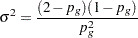 |
Tuning for the proposal  uses the following formula:
 |
where  is the standard deviation of the new proposal geometric distribution,
  is the standard deviation of the current proposal distribution, is the target acceptance probability, and is the current acceptance probability for the discrete parameter block.
The updated is the solution to the following equation that is between 0 and 1 :
 |
Binary Distribution: Independence Sampler
Blocks consisting of a single parameter with a binary prior do not require any tuning; the inverse-CDF method applies. Blocks that consist of multiple parameters with binary prior are sampled by using an independence sampler with binary proposal distributions. See the section Independence Sampler. During the tuning phase, the success probability of the proposal distribution is taken to be the probability of acceptance in the current loop. Ideally, an independence sampler works best if the acceptance rate is  , but that is rarely achieved. The algorithm stops when the probability of success exceeds the TARGACCEPTI=value, which has a default value of
  .
.
Footnotes
-
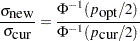
Roberts, Gelman, and Gilks (1997) and Roberts and Rosenthal (2001) demonstrate that the relationship between acceptance probability and scale in a random walk Metropolis is
 , where
  is the scale, is the acceptance rate,
  is the CDF of a standard normal, and
  ,
,  is the density function of samples. This relationship determines the updating scheme, with
  being replaced by the identity matrix to simplify calculation.