The MCMC Procedure
-
Overview

-
Getting Started
-
Syntax
-
Details
How PROC MCMC Works Blocking of Parameters Sampling Methods Tuning the Proposal Distribution Conjugate Sampling Initial Values of the Markov Chains Assignments of Parameters Standard Distributions Usage of Multivariate Distributions Specifying a New Distribution Using Density Functions in the Programming Statements Truncation and Censoring Some Useful SAS Functions Matrix Functions in PROC MCMC Create Design Matrix Modeling Joint Likelihood Regenerating Diagnostics Plots Caterpillar Plot Posterior Predictive Distribution Handling of Missing Data Floating Point Errors and Overflows Handling Error Messages Computational Resources Displayed Output ODS Table Names ODS Graphics
-
Examples
Simulating Samples From a Known Density Box-Cox Transformation Logistic Regression Model with a Diffuse Prior Logistic Regression Model with Jeffreys’ Prior Poisson Regression Nonlinear Poisson Regression Models Logistic Regression Random-Effects Model Nonlinear Poisson Regression Random-Effects Model Multivariate Normal Random-Effects Model Change Point Models Exponential and Weibull Survival Analysis Time Independent Cox Model Time Dependent Cox Model Piecewise Exponential Frailty Model Normal Regression with Interval Censoring Constrained Analysis Implement a New Sampling Algorithm Using a Transformation to Improve Mixing Gelman-Rubin Diagnostics
- References
Example 54.10 Change Point Models
Consider the data set from Bacon and Watts (1971), where  is the logarithm of the height of the stagnant surface layer and the covariate
  is the logarithm of the flow rate of water. The following statements create the data set:
title 'Change Point Model';
data stagnant;
   input y x @@;
   ind = _n_;
   datalines;
 1.12  -1.39   1.12  -1.39   0.99  -1.08   1.03  -1.08
 0.92  -0.94   0.90  -0.80   0.81  -0.63   0.83  -0.63
 0.65  -0.25   0.67  -0.25   0.60  -0.12   0.59  -0.12
 0.51   0.01   0.44   0.11   0.43   0.11   0.43   0.11
 0.33   0.25   0.30   0.25   0.25   0.34   0.24   0.34
 0.13   0.44  -0.01   0.59  -0.13   0.70  -0.14   0.70
-0.30   0.85  -0.33   0.85  -0.46   0.99  -0.43   0.99
-0.65   1.19
;
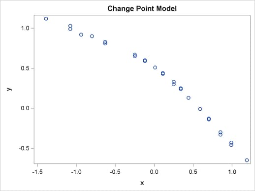
A scatter plot (Output 54.10.1) shows the presence of a nonconstant slope in the data. This suggests a change point regression model (Carlin, Gelfand, and Smith; 1992). The following statements generate the scatter plot in Output 54.10.1:
ods graphics on;
proc sgplot data=stagnant;
   scatter x=x y=y;
run;
Let the change point be cp. Following formulation by Spiegelhalter et al. (1996b), the regression model is as follows:
 |
You might consider the following diffuse prior distributions:
 |
 |
 |
|||
 |
|
 |
|||
 |
|
 |
The following statements generate Output 54.10.2:
proc mcmc data=stagnant outpost=postout seed=24860 ntu=1000
          nmc=20000;
   ods select PostSummaries;
   ods output PostSummaries=ds;

   array beta[2];
   parms alpha cp beta1 beta2;
   parms s2;

   prior cp ~ unif(-1.3, 1.1);
   prior s2  ~ uniform(0, 5);
   prior alpha beta:  ~ normal(0, v = 1e6);

   j = 1 + (x >= cp);
   mu = alpha + beta[j] * (x - cp);
   model y ~ normal(mu, var=s2);
run;
The PROC MCMC statement specifies the input data set (Stagnant), the output data set (Postout), a random number seed, a tuning sample of 1000, and an MCMC sample of 20000. The ODS SELECT statement displays only the summary statistics table. The ODS OUTPUT statement saves the summary statistics table to the data set Ds.
The ARRAY statement allocates an array of size 2 for the beta parameters. You can use beta1 and beta2 as parameter names without allocating an array, but having the array makes it easier to construct the likelihood function. The two PARMS statements put the five model parameters in two blocks. The three PRIOR statements specify the prior distributions for these parameters.
The symbol j indicates the segment component of the regression. When x is less than the change point, (x >= cp) returns 0 and j is assigned the value 1; if x is greater than or equal to the change point, (x >= cp) returns 1 and j is 2. The symbol mu is the mean for the jth segment, and beta[j] changes between the two regression coefficients depending on the segment component. The MODEL statement assigns the normal model to the response variable y.
Posterior summary statistics are shown in Output 54.10.2.
| Change Point Model |
| Posterior Summaries | ||||||
|---|---|---|---|---|---|---|
| Parameter | N | Mean | Standard Deviation |
Percentiles | ||
| 25% | 50% | 75% | ||||
| alpha | 20000 | 0.5349 | 0.0249 | 0.5188 | 0.5341 | 0.5509 |
| cp | 20000 | 0.0283 | 0.0314 | 0.00728 | 0.0303 | 0.0493 |
| beta1 | 20000 | -0.4200 | 0.0146 | -0.4293 | -0.4198 | -0.4111 |
| beta2 | 20000 | -1.0136 | 0.0167 | -1.0248 | -1.0136 | -1.0023 |
| s2 | 20000 | 0.000451 | 0.000145 | 0.000348 | 0.000425 | 0.000522 |
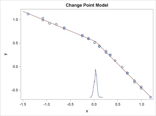
You can use PROC SGPLOT to visualize the model fit. Output 54.10.3 shows the fitted regression lines over the original data. In addition, on the bottom of the plot is the kernel density of the posterior marginal distribution of cp, the change point. The kernel density plot shows the relative variability of the posterior distribution on the data plot. You can use the following statements to create the plot:
data _null_;
   set ds;
   call symputx(parameter, mean);
run;

data b;
   missing A;
   input x1 @@;
   if x1 eq .A then x1 = &cp;
   if _n_ <= 2 then y1 = &alpha + &beta1 * (x1 - &cp);
   else y1 = &alpha + &beta2 * (x1 - &cp);
   datalines;
   -1.5 A 1.2
   ;

proc kde data=postout;
   univar cp / out=m1 (drop=count);
run;

data m1;
   set m1;
   density = (density / 25) - 0.653;
run;

data all;
   set stagnant b m1;
run;

proc sgplot data=all noautolegend;
   scatter x=x y=y;
   series x=x1 y=y1 / lineattrs = graphdata2;
   series x=value y=density / lineattrs = graphdata1;
run;
ods graphics off;
The macro variables &alpha, &beta1, &beta2, and &cp store the posterior mean estimates from the data set Ds. The data set Predicted contains three predicted values, at the minimum and maximum values of x and the estimated change point &cp. These input values give you fitted values from the regression model. Data set M1 contains the kernel density estimates of the parameter cp. The density is scaled down so the curve would fit in the plot. Finally, you use PROC SGPLOT to overlay the scatter plot, regression line and kernel density plots in the same graph.