The MCMC Procedure
-
Overview

-
Getting Started
-
Syntax
-
Details
How PROC MCMC Works Blocking of Parameters Sampling Methods Tuning the Proposal Distribution Conjugate Sampling Initial Values of the Markov Chains Assignments of Parameters Standard Distributions Usage of Multivariate Distributions Specifying a New Distribution Using Density Functions in the Programming Statements Truncation and Censoring Some Useful SAS Functions Matrix Functions in PROC MCMC Create Design Matrix Modeling Joint Likelihood Regenerating Diagnostics Plots Caterpillar Plot Posterior Predictive Distribution Handling of Missing Data Floating Point Errors and Overflows Handling Error Messages Computational Resources Displayed Output ODS Table Names ODS Graphics
-
Examples
Simulating Samples From a Known Density Box-Cox Transformation Logistic Regression Model with a Diffuse Prior Logistic Regression Model with Jeffreys’ Prior Poisson Regression Nonlinear Poisson Regression Models Logistic Regression Random-Effects Model Nonlinear Poisson Regression Random-Effects Model Multivariate Normal Random-Effects Model Change Point Models Exponential and Weibull Survival Analysis Time Independent Cox Model Time Dependent Cox Model Piecewise Exponential Frailty Model Normal Regression with Interval Censoring Constrained Analysis Implement a New Sampling Algorithm Using a Transformation to Improve Mixing Gelman-Rubin Diagnostics
- References
Example 54.4 Logistic Regression Model with Jeffreys’ Prior
A controlled experiment was run to study the effect of the rate and volume of air inspired on a transient reflex vasoconstriction in the skin of the fingers. Thirty-nine tests under various combinations of rate and volume of air inspired were obtained (Finney; 1947). The result of each test is whether or not vasoconstriction occurred. Pregibon (1981) uses this set of data to illustrate the diagnostic measures he proposes for detecting influential observations and to quantify their effects on various aspects of the maximum likelihood fit. The following statements create the data set Vaso:
title 'Logistic Regression Model with Jeffreys Prior';
data vaso;
   input vol rate resp @@;
   lvol = log(vol);
   lrate = log(rate);
   ind = _n_;
   cnst = 1;
   datalines;
3.7  0.825  1  3.5  1.09  1  1.25  2.5   1  0.75  1.5  1
0.8  3.2    1  0.7  3.5   1  0.6   0.75  0  1.1   1.7  0
0.9  0.75   0  0.9  0.45  0  0.8   0.57  0  0.55  2.75 0
0.6  3.0    0  1.4  2.33  1  0.75  3.75  1  2.3  1.64  1
3.2  1.6    1  0.85 1.415 1  1.7   1.06  0  1.8  1.8   1
0.4  2.0    0  0.95 1.36  0  1.35  1.35  0  1.5  1.36  0
1.6  1.78   1  0.6  1.5   0  1.8   1.5   1  0.95 1.9   0
1.9  0.95   1  1.6  0.4   0  2.7   0.75  1  2.35 0.03  0
1.1  1.83   0  1.1  2.2   1  1.2   2.0   1  0.8  3.33  1
0.95 1.9    0  0.75 1.9   0  1.3   1.625 1
;
The variable resp represents the outcome of a test. The variable lvol represents the log of the volume of air intake, and the variable lrate represents the log of the rate of air intake. You can model the data by using logistic regression. You can model the response with a binary likelihood:
 |
with
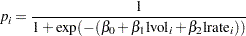 |
Let  be the design matrix in the regression. Jeffreys’ prior for this model is
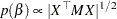 |
where  is a
is a  by matrix with off-diagonal elements being
  and diagonal elements being
  . For details on Jeffreys’ prior, see Jeffreys’ Prior. You can use a number of matrix functions, such as the determinant function, in PROC MCMC to construct Jeffreys’ prior. The following statements illustrate how to fit a logistic regression with Jeffreys’ prior:
%let n = 39;
proc mcmc data=vaso nmc=10000 outpost=mcmcout seed=17;
   ods select PostSummaries PostIntervals;

   array beta[3] beta0 beta1 beta2;
   array m[&n, &n];
   array x[1] / nosymbols;
   array xt[3, &n];
   array xtm[3, &n];
   array xmx[3, 3];
   array p[&n];

   parms beta0 1 beta1 1 beta2 1;

   begincnst;
      if (ind eq 1) then do;
         rc = read_array("vaso", x, "cnst", "lvol", "lrate");
         call transpose(x, xt);
         call zeromatrix(m);
      end;
   endcnst;

   beginnodata;
   call mult(x, beta, p);              /* p = x * beta */
   do i = 1 to &n;
      p[i] = 1 / (1 + exp(-p[i]));     /* p[i] = 1/(1+exp(-x*beta)) */
      m[i,i] = p[i] * (1-p[i]);
   end;
   call mult (xt, m, xtm);             /* xtm = xt * m        */
   call mult (xtm, x, xmx);            /* xmx = xtm * x       */
   call det (xmx, lp);                 /* lp = det(xmx)       */
   lp = 0.5 * log(lp);                 /* lp = -0.5 * log(lp) */
   prior beta: ~ general(lp);
   endnodata;

   model resp ~ bern(p[ind]);
run;
The first ARRAY statement defines an array beta with three elements: beta0, beta1, and beta2. The subsequent statements define arrays that are used in the construction of Jeffreys’ prior. These include m (the matrix), x (the design matrix), xt (the transpose of x), and some additional work spaces.
The explanatory variables lvol and lrate are saved in the array x in the BEGINCNST and ENDCNST statements. See BEGINCNST/ENDCNST Statement for details. After all the variables are read into x, you transpose the x matrix and store it to xt. The ZEROMATRIX function call assigns all elements in matrix m the value zero. To avoid redundant calculation, it is best to perform these calculations as the last observation of the data set is processed—that is, when ind is 39.
You calculate Jeffreys’ prior in the BEGINNODATA and ENDNODATA statements. The probability vector p is the product of the design matrix x and parameter vector beta. The diagonal elements in the matrix m are . The expression lp is the logarithm of Jeffreys’ prior. The PRIOR statement assigns lp as the prior for the  regression coefficients. The MODEL statement assigns a binary likelihood to resp, with probability p[ind]. The p array is calculated earlier using the matrix function MULT. You use the ind variable to pick out the right probability value for each resp.
Posterior summary statistics are displayed in Output 54.4.1.
| Logistic Regression Model with Jeffreys Prior |
| Posterior Summaries | ||||||
|---|---|---|---|---|---|---|
| Parameter | N | Mean | Standard Deviation |
Percentiles | ||
| 25% | 50% | 75% | ||||
| beta0 | 10000 | -2.9587 | 1.3258 | -3.8117 | -2.7938 | -2.0007 |
| beta1 | 10000 | 5.2905 | 1.8193 | 3.9861 | 5.1155 | 6.4145 |
| beta2 | 10000 | 4.6889 | 1.8189 | 3.3570 | 4.4914 | 5.8547 |
| Posterior Intervals | |||||
|---|---|---|---|---|---|
| Parameter | Alpha | Equal-Tail Interval | HPD Interval | ||
| beta0 | 0.050 | -5.8247 | -0.7435 | -5.5936 | -0.6027 |
| beta1 | 0.050 | 2.3001 | 9.3789 | 1.8590 | 8.7222 |
| beta2 | 0.050 | 1.6788 | 8.6643 | 1.3611 | 8.2490 |
You can also use PROC GENMOD to fit the same model by using the following statements:
proc genmod data=vaso descending;
   ods select PostSummaries PostIntervals;
   model resp = lvol lrate / d=bin link=logit;
   bayes seed=17 coeffprior=jeffreys nmc=20000 thin=2;
run;
The MODEL statement indicates that resp is the response variable and lvol and lrate are the covariates. The options in the MODEL statement specify a binary likelihood and a logit link function. The BAYES statement requests Bayesian capability. The SEED=, NMC=, and THIN= arguments work in the same way as in PROC MCMC. The COEFFPRIOR=JEFFREYS option requests Jeffreys’ prior in this analysis.
The PROC GENMOD statements produce Output 54.4.2, with estimates very similar to those reported in Output 54.4.1. Note that you should not expect to see identical output from PROC GENMOD and PROC MCMC, even with the simulation setup and identical random number seed. The two procedures use different sampling algorithms. PROC GENMOD uses the adaptive rejection metropolis algorithm (ARMS) (Gilks and Wild; 1992; Gilks; 2003) while PROC MCMC uses a random walk Metropolis algorithm. The asymptotic answers, which means that you let both procedures run an very long time, would be the same as they both generate samples from the same posterior distribution.
| Logistic Regression Model with Jeffreys Prior |
| Posterior Summaries | ||||||
|---|---|---|---|---|---|---|
| Parameter | N | Mean | Standard Deviation |
Percentiles | ||
| 25% | 50% | 75% | ||||
| Intercept | 10000 | -2.8731 | 1.3088 | -3.6754 | -2.7248 | -1.9253 |
| lvol | 10000 | 5.1639 | 1.8087 | 3.8451 | 4.9475 | 6.2613 |
| lrate | 10000 | 4.5501 | 1.8071 | 3.2250 | 4.3564 | 5.6810 |
| Posterior Intervals | |||||
|---|---|---|---|---|---|
| Parameter | Alpha | Equal-Tail Interval | HPD Interval | ||
| Intercept | 0.050 | -5.8246 | -0.7271 | -5.5774 | -0.6060 |
| lvol | 0.050 | 2.1844 | 9.2297 | 2.0112 | 8.9149 |
| lrate | 0.050 | 1.5666 | 8.6145 | 1.3155 | 8.1922 |