The MCMC Procedure
-
Overview

-
Getting Started
-
Syntax
-
Details
How PROC MCMC Works Blocking of Parameters Sampling Methods Tuning the Proposal Distribution Conjugate Sampling Initial Values of the Markov Chains Assignments of Parameters Standard Distributions Usage of Multivariate Distributions Specifying a New Distribution Using Density Functions in the Programming Statements Truncation and Censoring Some Useful SAS Functions Matrix Functions in PROC MCMC Create Design Matrix Modeling Joint Likelihood Regenerating Diagnostics Plots Caterpillar Plot Posterior Predictive Distribution Handling of Missing Data Floating Point Errors and Overflows Handling Error Messages Computational Resources Displayed Output ODS Table Names ODS Graphics
-
Examples
Simulating Samples From a Known Density Box-Cox Transformation Logistic Regression Model with a Diffuse Prior Logistic Regression Model with Jeffreys’ Prior Poisson Regression Nonlinear Poisson Regression Models Logistic Regression Random-Effects Model Nonlinear Poisson Regression Random-Effects Model Multivariate Normal Random-Effects Model Change Point Models Exponential and Weibull Survival Analysis Time Independent Cox Model Time Dependent Cox Model Piecewise Exponential Frailty Model Normal Regression with Interval Censoring Constrained Analysis Implement a New Sampling Algorithm Using a Transformation to Improve Mixing Gelman-Rubin Diagnostics
- References
Example 54.11 Exponential and Weibull Survival Analysis
This example covers two commonly used survival analysis models: the exponential model and the Weibull model. The deviance information criterion (DIC) is used to do model selections, and you can also find programs that visualize posterior quantities. Exponential and Weibull models are widely used for survival analysis. This example shows you how to use PROC MCMC to analyze the treatment effect for the E1684 melanoma clinical trial data. These data were collected to assess the effectiveness of using interferon alpha-2b in chemotherapeutic treatment of melanoma. The following statements create the data set:
data e1684;
   input t t_cen treatment @@;
   if t = . then do;
     t = t_cen;
     v = 0;
   end;
   else
     v = 1;
   ifn = treatment - 1;
   et = exp(t);
   lt = log(t);
   drop t_cen;
   datalines;
 1.57808  0.00000  2   1.48219  0.00000  2    .       7.33425  1
 2.23288  0.00000  1    .       9.38356  2   3.27671  0.00000  1
  .       9.64384  1   1.66575  0.00000  2   0.94247  0.00000  1

   ... more lines ...

 3.39178  0.00000  1   .        4.36164  2   .        4.81918  2
;
The data set E1684 contains the following variables: t is the failure time that equals the censoring time whether the observation was censored, v indicates whether the observation is an actual failure time or a censoring time, treatment indicates two levels of treatments, and ifn indicates the use of interferon as a treatment. The variables et and lt are the exponential and logarithm transformation of the time t. The published data contains other potential covariates that are not listed here. This example concentrates on the effectiveness of the interferon treatment.
Exponential Survival Model
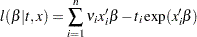
The density function for exponentially distributed survival times is as follows:
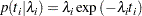 |
Note that this formulation of the exponential distribution is different from what is used in the SAS probability function PDF. The definition used in PDF for the exponential distributions is as follows:
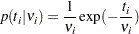 |
The relationship between  and
and  is as follows:
 |
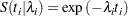
The corresponding survival function, using the  formulation, is as follows:
 |
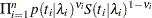
If you have a sample  of
of  independent exponential survival times, each with mean , then the likelihood function in terms of is as follows:
 |
 |
 |
|||
 |
|
 |
|||
|
|
 |
If you link the covariates to with  , where
  is the vector of covariates corresponding to the
  th observation and
  is a vector of regression coefficients, then the log-likelihood function is as follows:
 |
In the absence of prior information about the parameters in this model, you can choose diffuse normal priors for the :
 |
There are two ways to program the log-likelihood function in PROC MCMC. You can use the SAS functions LOGPDF and LOGSDF. Alternatively, you can use the simplified log-likelihood function, which is more computationally efficient. You get identical results by using either approaches.
The following PROC MCMC statements fit an exponential model with simplified log-likelihood function:
title 'Exponential Survival Model';
ods graphics on;
proc mcmc data=e1684 outpost=expsurvout nmc=10000 seed=4861;
    ods select PostSummaries PostIntervals TADpanel
               ess mcse;
   parms (beta0 beta1) 0;
   prior beta: ~ normal(0, sd = 10000);
   /*****************************************************/
   /* (1) the logpdf and logsdf functions are not used  */
   /*****************************************************/
   /*     nu = 1/exp(beta0 + beta1*ifn);
          llike = v*logpdf("exponential", t, nu) +
                  (1-v)*logsdf("exponential", t, nu);
   */
   /****************************************************/
   /* (2) the simplified likelihood formula is used    */
   /****************************************************/
   l_h = beta0 + beta1*ifn;
   llike = v*(l_h) -  t*exp(l_h);
   model general(llike);
run;
The two assignment statements that are commented out calculate the log-likelihood function by using the SAS functions LOGPDF and LOGSDF for the exponential distribution. The next two assignment statements calculate the log likelihood by using the simplified formula. The first approach is slower because of the redundant calculation involved in calling both LOGPDF and LOGSDF.
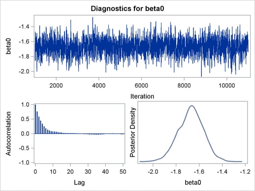
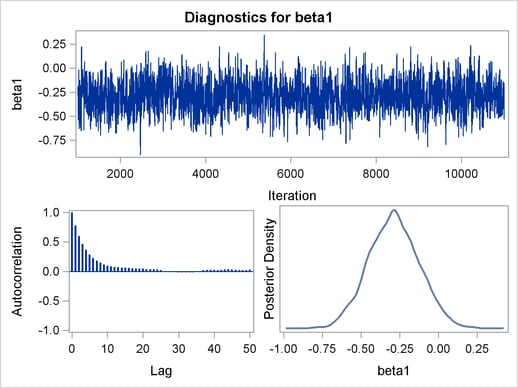
An examination of the trace plots for  and
and  (see Output 54.11.1) reveals that the sampling has gone well with no particular concerns about the convergence or mixing of the chains.
and in the Exponential Survival Analysis
The MCMC results are shown in Output 54.11.2.
| Exponential Survival Model |
| Posterior Summaries | ||||||
|---|---|---|---|---|---|---|
| Parameter | N | Mean | Standard Deviation |
Percentiles | ||
| 25% | 50% | 75% | ||||
| beta0 | 10000 | -1.6715 | 0.1091 | -1.7426 | -1.6684 | -1.5964 |
| beta1 | 10000 | -0.2879 | 0.1615 | -0.4001 | -0.2892 | -0.1803 |
| Posterior Intervals | |||||
|---|---|---|---|---|---|
| Parameter | Alpha | Equal-Tail Interval | HPD Interval | ||
| beta0 | 0.050 | -1.8907 | -1.4639 | -1.8930 | -1.4673 |
| beta1 | 0.050 | -0.5985 | 0.0300 | -0.6104 | 0.0169 |
The Monte Carlo standard errors and effective sample sizes are shown in Output 54.11.3. The posterior means for and are estimated with high precision, with small standard errors with respect to the standard deviation. This indicates that the mean estimates have stabilized and do not vary greatly in the course of the simulation. The effective sample sizes are roughly the same for both parameters.
| Exponential Survival Model |
| Monte Carlo Standard Errors | |||
|---|---|---|---|
| Parameter | MCSE | Standard Deviation |
MCSE/SD |
| beta0 | 0.00302 | 0.1091 | 0.0277 |
| beta1 | 0.00485 | 0.1615 | 0.0301 |
| Effective Sample Sizes | |||
|---|---|---|---|
| Parameter | ESS | Autocorrelation Time |
Efficiency |
| beta0 | 1304.1 | 7.6682 | 0.1304 |
| beta1 | 1107.2 | 9.0319 | 0.1107 |
The next part of this example shows fitting a Weibull regression to the data and then comparing the two models with DIC to see which one provides a better fit to the data.
Weibull Survival Model
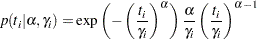
The density function for Weibull distributed survival times is as follows:
 |
Note that this formulation of the Weibull distribution is different from what is used in the SAS probability function PDF. The definition used in PDF is as follows:
 |
The relationship between and  in these two parameterizations is as follows:
 |
The corresponding survival function, using the formulation, is as follows:
 |
If you have a sample of independent Weibull survival times, with parameters  , and , then the likelihood function in terms of and is as follows:
 |
|
 |
|||
|
|
 |
|||
|
|
 |
If you link the covariates to with  , where is the vector of covariates corresponding to the th observation and is a vector of regression coefficients, the log-likelihood function becomes this:
 |
As with the exponential model, in the absence of prior information about the parameters in this model, you can use diffuse normal priors on  You might want to choose a diffuse gamma distribution for
  Note that when
  , the Weibull survival likelihood reduces to the exponential survival likelihood. Equivalently, by looking at the posterior distribution of , you can conclude whether fitting an exponential survival model would be more appropriate than the Weibull model.
PROC MCMC also enables you to make inference on any functions of the parameters. Quantities of interest in survival analysis include the value of the survival function at specific times for specific treatments and the relationship between the survival curves for different treatments. With PROC MCMC, you can compute a sample from the posterior distribution of the interested survival functions at any number of points. The data in this example range from about 0 to 10 years, and the treatment of interest is the use of interferon.
Like in the previous exponential model example, there are two ways to fit this model: using the SAS functions LOGPDF and LOGSDF, or using the simplified log likelihood functions. The example uses the latter method. The following statements run PROC MCMC and produce Output 54.11.4:
title 'Weibull Survival Model';
proc mcmc data=e1684 outpost=weisurvout nmc=10000 seed=1234
          monitor=(_parms_ surv_ifn surv_noifn);
   ods select PostSummaries;
   ods output PostSummaries=ds PostIntervals=is;
   array surv_ifn[10];
   array surv_noifn[10];
   parms alpha 1 (beta0 beta1) 0;
   prior beta: ~ normal(0, var=10000);
   prior alpha ~ gamma(0.001,is=0.001);

   beginnodata;
      do t1 = 1 to 10;
        surv_ifn[t1] = exp(-exp(beta0+beta1)*t1**alpha);
        surv_noifn[t1] = exp(-exp(beta0)*t1**alpha);
      end;
   endnodata;

   lambda = beta0 + beta1*ifn;
   /*****************************************************/
   /* (1) the logpdf and logsdf functions are not used  */
   /*****************************************************/
   /*     gamma =  exp(-lambda /alpha);
          llike = v*logpdf('weibull', t, alpha, gamma) +
                  (1-v)*logsdf('weibull', t, alpha, gamma);
   */
   /****************************************************/
   /* (2) the simplified likelihood formula is used    */
   /****************************************************/
   llike  = v*(log(alpha) + (alpha-1)*log(t) + lambda) -
            exp(lambda)*(t**alpha);
   model general(llike);
run;
The MONITOR= option indicates the parameters and quantities of interest that PROC MCMC tracks. The symbol _PARMS_ specifies all model parameters. The array surv_ifn stores the expected survival probabilities for patients who received interferon over a period of 10 years. Similarly, surv_noifn stores the expected survival probabilities for patients who did not received interferon.
The BEGINNODATA and ENDNODATA statements enclose the calculations for the survival probabilities. The assignment statements proceeding the MODEL statement calculate the log likelihood for the Weibull survival model. The MODEL statement specifies the log likelihood that you programmed.
An examination of the trace plots for , , and (not displayed here) reveals that the sampling has gone well, with no particular concerns about the convergence or mixing of the chains.
Output 54.11.4 displays the posterior summary statistics.
| Weibull Survival Model |
| Posterior Summaries | ||||||
|---|---|---|---|---|---|---|
| Parameter | N | Mean | Standard Deviation |
Percentiles | ||
| 25% | 50% | 75% | ||||
| alpha | 10000 | 0.7891 | 0.0539 | 0.7514 | 0.7880 | 0.8260 |
| beta0 | 10000 | -1.3581 | 0.1369 | -1.4519 | -1.3597 | -1.2624 |
| beta1 | 10000 | -0.2512 | 0.1541 | -0.3541 | -0.2606 | -0.1521 |
| surv_ifn1 | 10000 | 0.8175 | 0.0227 | 0.8027 | 0.8187 | 0.8331 |
| surv_ifn2 | 10000 | 0.7066 | 0.0291 | 0.6874 | 0.7072 | 0.7265 |
| surv_ifn3 | 10000 | 0.6203 | 0.0331 | 0.5983 | 0.6205 | 0.6436 |
| surv_ifn4 | 10000 | 0.5495 | 0.0360 | 0.5253 | 0.5497 | 0.5747 |
| surv_ifn5 | 10000 | 0.4899 | 0.0381 | 0.4635 | 0.4895 | 0.5170 |
| surv_ifn6 | 10000 | 0.4390 | 0.0396 | 0.4118 | 0.4382 | 0.4666 |
| surv_ifn7 | 10000 | 0.3949 | 0.0406 | 0.3669 | 0.3934 | 0.4223 |
| surv_ifn8 | 10000 | 0.3564 | 0.0413 | 0.3281 | 0.3551 | 0.3840 |
| surv_ifn9 | 10000 | 0.3225 | 0.0416 | 0.2940 | 0.3212 | 0.3505 |
| surv_ifn10 | 10000 | 0.2926 | 0.0416 | 0.2638 | 0.2911 | 0.3208 |
| surv_noifn1 | 10000 | 0.7719 | 0.0274 | 0.7535 | 0.7736 | 0.7913 |
| surv_noifn2 | 10000 | 0.6401 | 0.0339 | 0.6171 | 0.6415 | 0.6635 |
| surv_noifn3 | 10000 | 0.5415 | 0.0374 | 0.5161 | 0.5428 | 0.5662 |
| surv_noifn4 | 10000 | 0.4635 | 0.0395 | 0.4365 | 0.4636 | 0.4890 |
| surv_noifn5 | 10000 | 0.4001 | 0.0406 | 0.3725 | 0.3995 | 0.4261 |
| surv_noifn6 | 10000 | 0.3475 | 0.0411 | 0.3195 | 0.3459 | 0.3745 |
| surv_noifn7 | 10000 | 0.3034 | 0.0411 | 0.2758 | 0.3012 | 0.3299 |
| surv_noifn8 | 10000 | 0.2661 | 0.0406 | 0.2384 | 0.2630 | 0.2921 |
| surv_noifn9 | 10000 | 0.2342 | 0.0399 | 0.2069 | 0.2311 | 0.2592 |
| surv_noifn10 | 10000 | 0.2069 | 0.0389 | 0.1803 | 0.2035 | 0.2312 |
An examination of the parameter reveals that the exponential model might not be inappropriate here. The estimated posterior mean of is 0.7856 with a posterior standard deviation of 0.0533. As noted previously, if , then the Weibull survival distribution is the exponential survival distribution. With these data, you can see that the evidence is in favor of  . The value 1 is almost 4 posterior standard deviations away from the posterior mean. The following statements compute the posterior probability of the hypothesis that
  :
:
proc format;
   value alphafmt low-<1 = 'alpha < 1' 1-high = 'alpha >= 1';
run;

proc freq data=weisurvout;
   tables alpha /nocum;
   format alpha alphafmt.;
run;
The PROC FREQ results are shown in Output 54.11.5.
| Weibull Survival Model |
| alpha | Frequency | Percent |
|---|---|---|
| alpha < 1 | 9998 | 99.98 |
| alpha >= 1 | 2 | 0.02 |
The output from PROC FREQ shows that 100% of the 10000 simulated values for are less than 1. This is a very strong indication that the exponential model is too restrictive to model these data well.
You can examine the estimated survival probabilities over time individually, either through the posterior summary statistics or by looking at the kernel density plots. Alternatively, you might find it more informative to examine these quantities in relation with each other. For example, you can use a side-by-side box plot to display these posterior distributions by using PROC SGPLOT (Statistical Graphics Using ODS). First you need to take the posterior output data set Weisurvout and stack variables that you want to plot. For example, to plot all the survival times for patients who received interferon, you want to stack surv_inf1–surv_inf10. The macro %Stackdata takes an input data set dataset, stacks the wanted variables vars, and outputs them into the output data set.
The following statements define the macro stackdata:
/* define macro stackdata */
%macro StackData(dataset,output,vars);
   data &output;
      length var $ 32;
      if 0 then set &dataset nobs=nnn;
      array lll[*] &vars;
      do jjj=1 to dim(lll);
         do iii=1 to nnn;
            set &dataset point=iii;
            value = lll[jjj];
            call vname(lll[jjj],var);
            output;
         end;
      end;
      stop;
      keep var value;
   run;
%mend;

/* stack the surv_ifn variables and saved them to survifn. */
%StackData(weisurvout, survifn, surv_ifn1-surv_ifn10);
Once you stack the data, use PROC SGPLOT to create the side-by-side box plots. The following statements generate Output 54.11.6:
proc sgplot data=survifn;
   yaxis label='Survival Probability' values=(0 to 1 by 0.2);
   xaxis label='Time' discreteorder=data;
   vbox value / category=var;
run;
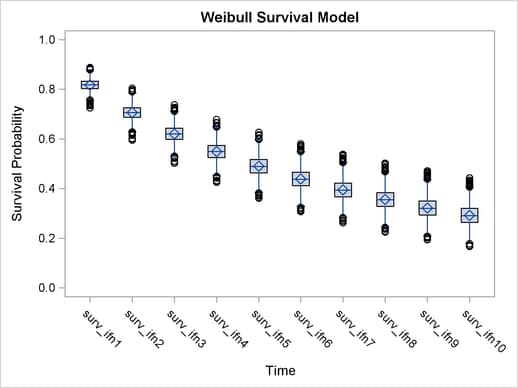
There is a clear decreasing trend over time of the survival probabilities for patients who receive the treatment. You might ask how does this group compare to those who did not receive the treatment? In this case, you want to overlay the two predicted curves for the two groups of patients and add the corresponding credible interval. See Output 54.11.7. To generate the graph, you first take the posterior mean estimates from the ODS output table ds and the lower and upper HPD interval estimates is, store them in the data set Surv, and draw the figure by using PROC SGPLOT.
The following statements generate data set Surv:
data surv;
   set ds;
   if _n_ >= 4 then do;
      set is point=_n_;
      group = 'with interferon   ';
      time = _n_ - 3;
      if time > 10 then do;
         time = time - 10;
         group = 'without interferon';
      end;
      output;
   end;
   keep time group mean hpdlower hpdupper;
run;
The following SGPLOT statements generate Output 54.11.7:
proc sgplot data=surv;
   yaxis label="Survival Probability" values=(0 to 1 by 0.2);
   series x=time y=mean / group = group name='i';
   band x=time lower=hpdlower upper=hpdupper / group = group transparency=0.7;
   keylegend 'i';
run;
ods graphics off;
In Output 54.11.7, the solid line is the survival curve for patients who received interferon; the shaded region centers at the solid line is the 95% HPD intervals; the medium-dashed line is the survival curve for patients who did not receive interferon; and the shaded region around the dashed line is the corresponding 95% HPD intervals.
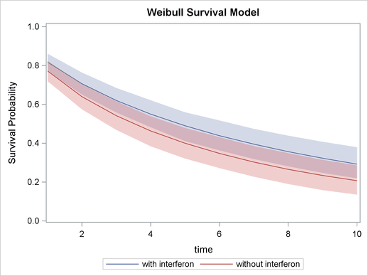
The plot suggests that there is an effect of using interferon because patients who received interferon have sustained better survival probabilities than those who did not. However, the effect might not be very significant, as the 95% credible intervals of the two groups do overlap. For more on these interferon studies, refer to Ibrahim, Chen, and Sinha (2001).
Weibull or Exponential?
Although the evidence from the Weibull model fit shows that the posterior distribution of has a significant amount of density mass less than 1, suggesting that the Weibull model is a better fit to the data than the exponential model, you might still be interested in comparing the two models more formally. You can use the Bayesian model selection criterion (see the section Deviance Information Criterion (DIC)) to determine which model fits the data better.
The PROC MCMC DIC option requests the calculation of DIC, and the procedure displays the ODS output table DIC. The table includes the posterior mean of the deviation,  , deviation at the estimate,
  , effective number of parameters,
  , and DIC. It is important to remember that the standardizing term,
  , which is a function of the data alone, is not taken into account in calculating the DIC. This term is irrelevant only if you compare two models that have the same likelihood function. If you do not have identical likelihood functions, using DIC for model selection purposes without taking this standardizing term into account can produce incorrect results. In addition, you want to be careful in interpreting the DIC whenever you use the GENERAL function to construct the log-likelihood, as the case in this example. Using the GENERAL function, you can obtain identical posterior samples with two log-likelihood functions that differ only by a constant. This difference translates to a difference in the DIC calculation, which could be very misleading.
If  , the Weibull likelihood is identical to the exponential likelihood. It is safe in this case to directly compare DICs from these two models. However, if you do not want to work out the mathematical detail or you are uncertain of the equivalence, a better way of comparing the DICs is to run the Weibull model twice: once with being a parameter and once with . This ensures that the likelihood functions are the same, and the DIC comparison is meaningful.
The following statements fit a Weibull model:
title 'Model Comparison between Weibull and Exponential';
proc mcmc data=e1684 outpost=weisurvout nmc=10000 seed=4861 dic;
   ods select dic;
   parms alpha 1 (beta0 beta1) 0;
   prior beta: ~ normal(0, var=10000);
   prior alpha ~ gamma(0.001,is=0.001);

   lambda = beta0 + beta1*ifn;
   llike  = v*(log(alpha) + (alpha-1)*log(t) + lambda) -
            exp(lambda)*(t**alpha);
   model general(llike);
run;
The DIC option requests the calculation of DIC, and the table is displayed is displayed in Output 54.11.8:
| Model Comparison between Weibull and Exponential |
| Deviance Information Criterion | |
|---|---|
| Dbar (posterior mean of deviance) | 858.623 |
| Dmean (deviance evaluated at posterior mean) | 855.633 |
| pD (effective number of parameters) | 2.990 |
| DIC (smaller is better) | 861.614 |
| The GENERAL or DGENERAL function is used in this program. To make meaningful comparisons, you must ensure that all GENERAL or DGENERAL functions include appropriate normalizing constants. Otherwise, DIC comparisons can be misleading. | |
The note in Output 54.11.8 reminds you of the importance of ensuring identical likelihood functions when you use the GENERAL function. The DIC value is  .
.
Based on the same set of code, the following statements fit an exponential model by setting :
proc mcmc data=e1684 outpost=expsurvout nmc=10000 seed=4861 dic;
   ods select dic;
   parms beta0 beta1 0;
   prior beta: ~ normal(0, var=10000);
   begincnst;
      alpha = 1;
   endcnst;

   lambda = beta0 + beta1*ifn;
   llike  = v*(log(alpha) + (alpha-1)*log(t) + lambda) -
            exp(lambda)*(t**alpha);
   model general(llike);
run;
Output 54.11.9 displays the DIC table.
| Model Comparison between Weibull and Exponential |
| Deviance Information Criterion | |
|---|---|
| Dbar (posterior mean of deviance) | 870.133 |
| Dmean (deviance evaluated at posterior mean) | 868.190 |
| pD (effective number of parameters) | 1.943 |
| DIC (smaller is better) | 872.075 |
| The GENERAL or DGENERAL function is used in this program. To make meaningful comparisons, you must ensure that all GENERAL or DGENERAL functions include appropriate normalizing constants. Otherwise, DIC comparisons can be misleading. | |
The DIC value of  is greater than
  . A smaller DIC indicates a better fit to the data; hence, you can conclude that the Weibull model is more appropriate for this data set. You can see the equivalencing of the exponential model you fitted in Exponential Survival Model by running the following comparison.
The following statements are taken from the section Exponential Survival Model, and they fit the same exponential model:
proc mcmc data=e1684 outpost=expsurvout1 nmc=10000 seed=4861 dic;
   ods select none;
   parms (beta0 beta1) 0;
   prior beta: ~ normal(0, sd = 10000);
   l_h = beta0 + beta1*ifn;
   llike = v*(l_h) -  t*exp(l_h);
   model general(llike);
run;

proc compare data=expsurvout compare=expsurvout1;
   var beta0 beta1;
run;
The posterior samples of beta0 and beta1 in the data set Expsurvout1 are identical to those in the data set Expsurvout. The comparison results are not shown here.