The MCMC Procedure
-
Overview

-
Getting Started
-
Syntax
-
Details
How PROC MCMC Works Blocking of Parameters Sampling Methods Tuning the Proposal Distribution Conjugate Sampling Initial Values of the Markov Chains Assignments of Parameters Standard Distributions Usage of Multivariate Distributions Specifying a New Distribution Using Density Functions in the Programming Statements Truncation and Censoring Some Useful SAS Functions Matrix Functions in PROC MCMC Create Design Matrix Modeling Joint Likelihood Regenerating Diagnostics Plots Caterpillar Plot Posterior Predictive Distribution Handling of Missing Data Floating Point Errors and Overflows Handling Error Messages Computational Resources Displayed Output ODS Table Names ODS Graphics
-
Examples
Simulating Samples From a Known Density Box-Cox Transformation Logistic Regression Model with a Diffuse Prior Logistic Regression Model with Jeffreys’ Prior Poisson Regression Nonlinear Poisson Regression Models Logistic Regression Random-Effects Model Nonlinear Poisson Regression Random-Effects Model Multivariate Normal Random-Effects Model Change Point Models Exponential and Weibull Survival Analysis Time Independent Cox Model Time Dependent Cox Model Piecewise Exponential Frailty Model Normal Regression with Interval Censoring Constrained Analysis Implement a New Sampling Algorithm Using a Transformation to Improve Mixing Gelman-Rubin Diagnostics
- References
Example 54.1 Simulating Samples From a Known Density
This example illustrates how you can obtain random samples from a known function. The target distributions are the normal distribution and a mixture of the normal distributions. You do not need any input data set to generate samples from a known density. You can set the likelihood function to a constant. The posterior distribution becomes identical to the prior distributions that you specify.
Sampling from a Normal Density
With a constant likelihood, there is no need to input a response variable since no data are relevant to a flat likelihood. However, PROC MCMC requires an input data set, so you can use an empty data set as the input data set. The following statements generate 10000 samples from a standard normal distribution:
title 'Simulating Samples from a Normal Density';
data x;
run;

ods graphics on;
proc mcmc data=x outpost=simout seed=23 nmc=10000 maxtune=0
          nbi=0 statistics=(summary interval) diagnostics=none;
   ods exclude nobs parameters;
   parm alpha 0;
   prior alpha ~ normal(0, sd=1);
   model general(0);
run;
The ODS GRAPHICS ON statement enables ODS Graphics. The PROC MCMC statement specifies the input and output data sets, a random number seed, and the size of the simulation sample. There is no need for tuning (MAXTUNE=0) because the default scale and the proposal variance are optimal for a standard normal target distribution. For the same reason, no burn-in is needed (NBI=0). The STATISTICS= option is used to display only the summary and interval statistics. The ODS EXCLUDE statement excludes the display of the NObs and Parameters tables. The summary statistics (Output 54.1.1) are what you would expect from a standard normal distribution.
| Simulating Samples from a Normal Density |
| Posterior Summaries | ||||||
|---|---|---|---|---|---|---|
| Parameter | N | Mean | Standard Deviation |
Percentiles | ||
| 25% | 50% | 75% | ||||
| alpha | 10000 | -0.0392 | 1.0194 | -0.7198 | -0.0403 | 0.6351 |
| Posterior Intervals | |||||
|---|---|---|---|---|---|
| Parameter | Alpha | Equal-Tail Interval | HPD Interval | ||
| alpha | 0.050 | -2.0746 | 1.9594 | -2.2197 | 1.7869 |
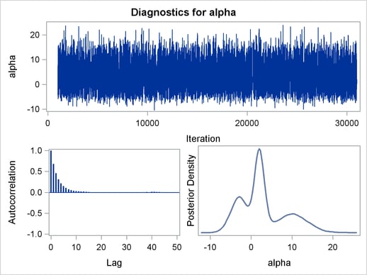
The trace plot (Output 54.1.2) shows good mixing of the Markov chain, and there is no significant autocorrelation in the lag plot.

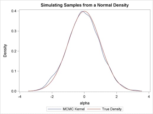
You can also overlay the estimated kernel density with the true density to get a visual comparison, as displayed in Output 54.1.3.
To create Output 54.1.3, you first use PROC KDE (see Chapter 47, The KDE Procedure ) to obtain a kernel density estimate of the posterior density on alpha, and then you evaluate a grid of alpha values by using PROC KDE output data set Sample on a normal density. The following statements evaluate kernel density and compute corresponding normal density.
proc kde data=simout;
   ods exclude inputs controls;
   univar alpha /out=sample;
run;

data den;
   set sample;
   alpha = value;
   true  = pdf('normal', alpha, 0, 1);
   keep alpha density true;
run;
Finally, you plot the two curves on top of each other by using PROC SGPLOT (see Chapter 21, Statistical Graphics Using ODS ); the resulting figure is in Output 54.1.3. You can see that the kernel estimate and the true density are very similar to one another. The following statements produce Output 54.1.3:
proc sgplot data=den;
   yaxis label="Density";
   series y=density x=alpha / legendlabel = "MCMC Kernel";
   series y=true x=alpha / legendlabel = "True Density";
   discretelegend;
run;
Sampling from a Mixture of Normal Densities
Suppose that you are interested in generating samples from a three-component mixture of normal distributions, with the density specified as follows:
 |
The following statements generate random samples from this mixture density:
title 'Simulating Samples from a Mixture of Normal Densities';
data x;
run;

proc mcmc data=x outpost=simout seed=1234 nmc=30000;
   ods select TADpanel;
   parm alpha 0.3;
   lp = logpdf('normalmix', alpha, 3, 0.3, 0.4, 0.3, -3, 2, 10, 2, 1, 4);
   prior alpha  ~ general(lp);
   model general(0);
run;
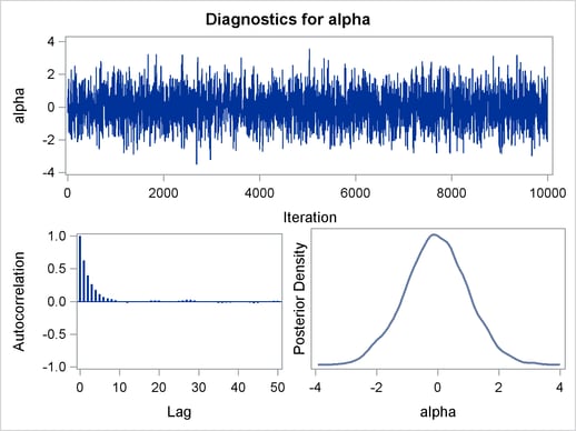
The ODS SELECT statement displays the diagnostic plots. All other tables, such as the NObs tables, are excluded. The PROC MCMC statement uses the input data set X, saves output to the Simout data set, sets a random number seed, and simulates 30,000 samples.
The lp assignment statement evaluates the log density of alpha at the mixture density, using the SAS function LOGPDF. The number 3 after alpha in the LOGPDF function indicates that the density is a three-component normal mixture. The following three numbers,  ,
,  , and , are the weights in the mixture;
  ,
,  , and
, and  are the means; ,
  , and
, and  are the standard deviations. The PRIOR statement assigns this log density function to alpha as its prior. Note that the GENERAL function interprets the density on the log scale, and not the original scale. Hence, you must use the LOGPDF function, not the PDF function. Output 54.1.4 displays the results. The kernel density clearly shows three modes.
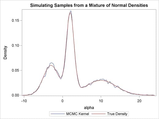
Using the following set of statements similar to the previous example, you can overlay the estimated kernel density with the true density. The comparison is shown in Output 54.1.5.
proc kde data=simout;
   ods exclude inputs controls;
   univar alpha /out=sample;
run;

data den;
   set sample;
   alpha = value;
   true  = pdf('normalmix', alpha, 3, 0.3, 0.4, 0.3, -3, 2, 10, 2, 1, 4);
   keep alpha density true;
run;

proc sgplot data=den;
   yaxis label="Density";
   series y=density x=alpha / legendlabel = "MCMC Kernel";
   series y=true x=alpha / legendlabel = "True Density";
   discretelegend;
run;
ods graphics off;