The MCMC Procedure

Density Functions in PROC MCMC

PROC MCMC has a number of internally defined log-density functions for univariate and multivariate distributions. These functions have the basic form of LPDFdist(x, parm-list), where dist is the name of the distribution (see Table 54.39 for univariate distributions and Table 54.40 for multivariate distributions). The argument x is the random variable, and parm-list is the list of parameters.

In addition, the univariate functions allow for optional boundary arguments, such as LPDFdist(x, parm-list, <lower>, <upper>), where lower and upper are optional but positional boundary arguments. With the exception of the Bernoulli and uniform distribution, you can specify limits on all univariate distributions.

To set a lower bound on the normal density:

lpdfnorm(x, 0, 1, -2);

To set just an upper bound, specify a missing value for the lower bound argument:

lpdfnorm(x, 0, 1, ., 2);

Leaving both limits out gives you the unbounded density. You can also specify both bounds:

lpdfnorm(x, 0, 1);
lpdfnorm(x, 0, 1, -3, 4);

See Table 54.39 for the function names of univariate distributions and Table 54.40 for multivariate distributions.

In the multivariate log-density functions, arrays must be used in place for the random variable and parameters in the model.

Standard Distributions, the LOGPDF Functions, and the LPDFdist Functions

Standard distributions listed in the section Standard Distributions are names only, and they can be used only in the MODEL, PRIOR, and HYPERPRIOR statements to specify either a prior distribution or a conditional distribution of the data given parameters. They do not return any values, and you cannot use them in the programming statements.

The LOGPDF functions are DATA step functions that compute the logarithm of various probability density (mass) functions. For example, logpdf("beta", x, 2, 15) returns the log of a beta density with parameters a = 2 and b = 15, evaluated at . All the LOGPDF functions are supported in PROC MCMC.

The LPDFdist functions are unique to PROC MCMC. They compute the logarithm of various probability density (mass) functions. The functions are the same as the LOGPDF functions when it comes to calculating the log density. For example, lpdfbeta(x, 2, 15) returns the same value as logpdf("beta", x, 2, 15). The LPDFdist functions cover a greater class of probability density functions, and the univariate distribution functions take the optional but positional boundary arguments. There are no corresponding LCDFdist or LSDFdist functions in PROC MCMC. To work with the cumulative probability function or the survival functions, you need to use the LOGCDF and the LOGSDF DATA step functions.

Multivariate Density Functions in the Data Step

The DATA step has functions that compute the logarithm of the density of some multivariate distributions. You can also use them in PROC MCMC. For a complete listing of multivariate functions, see SAS Language Reference: Dictionary.

Some commonly used multivariate functions are as follows:

• LOGMPDFNORMAL, the logarithm of the multivariate normal

• LOGMPDFWISHART, the logarithm of the Wishart

• LOGMPDFIWISHART, the logarithm of the inverted-Wishart

• LOGMPDFDIR1, the logarithm of the Dirichlet distribution of Type I

• LOGMPDFDIR2, the logarithm of the Dirichlet distribution of Type II

• LOGMPDFMULTINOM, the logarithm of the multinomial

Other multivariate density functions include: LOGMPDFT (t distribution), LOGMPDFGAMMA (gamma distribution), LOGMPDFBETA1 (beta of type I), and LOGMPDFBETA2 (beta of type II).

Density Function Definition

LOGMPDFNORMAL

Let be an -dimensional random vector with mean vector and covariance matrix . The density is

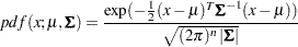where is the determinant of the covariance matrix .

The function has syntax:

Warning: you must set up the covariance matrix before using the LOGMPDFNORMAL function and free the memory after PROC MCMC exits. See the section Set Up the Covariance Matrices and Free Memory.

LOGMPDFWISHART and LOGMPDFIWISHART

The density function from the Wishart distribution is:

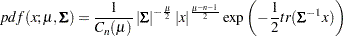with , and the trace of a square matrix is given by:

The density function from the inverse-Wishart distribution is:

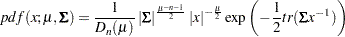for , and

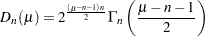If then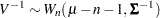

The functions have syntax:

and for the inverted Wishart:

The three arguments are the multivariate matrix , the degrees of freedom , and the covariance matrix k

Warning: you must set up the covariance matrix before using these functions and free the memory after PROC MCMC exits. See the section Set Up the Covariance Matrices and Free Memory.

LOGMPDFDIR1 and LOGMPDFDIR2

The random variables , with and , are said to have a Dirichlet Type I distribution with parameters if their joint pdf is given by:

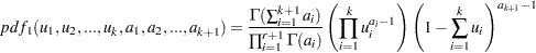The variables are said to have a Dirichlet type II distribution with parameters if their joint pdf is given by the following:

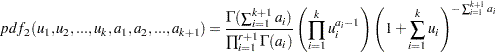The functions have syntax:

and

LOGMPDFMULTINOM

Let be random variables that denote the number of occurring of the events respectively occurring with probabilities . Let and let . Then the joint distribution of is the following:

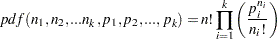The function has syntax:

Set Up the Covariance Matrices and Free Memory

For distributions that require symmetric positive definite matrices, such as the LOGMPDFNORMAL, LOGMPDFWISHART and LOGMPDFIWISHART functions, you need to set up these matrices by using the following functions:

• Use LOGMPDFSETSQ to set up a symmetric positive definite matrix from all its elements:

  is set to when the numeric arguments describe a symmetric positive definite matrix, otherwise it is set to a nonzero value.

• Use LOGMPDFSET to set up a symmetric positive definite matrix from its lower triangular elements:

  When the numeric arguments describe a symmetric positive definite matrix, the returned value is set to . Otherwise, a nonzero value for is returned.

• Use LOGMPFFREE to free the workspace previously allocated with either LOGMPDFSET or LOGMPDFSETSQ:

  When called without arguments, the LOGMPDFFREE frees all the symbols previously allocated by LOGMPDFSETSQ or LOGMPDFSET. Each freed symbol is reported back in the SAS log.

The parameters used in these functions are defined as follows:

• is a string containing the name of the work space that stores the matrix by the numeric parameters .

• are numeric arguments that represent the elements of a symmetric positive definite matrix.

You would set up this matrix under the DATA step by using the following syntax:

or the syntax:

If the matrix is positive definite, the returned value is zero.