The MCMC Procedure

Posterior Predictive Distribution

The posterior predictive distribution

$\text{[math]}$

can often be used to check whether the model is consistent with data. For more information about using predictive distribution as a model checking tool, see Gelman et al.; 2004, Chapter 6 and the bibliography in that chapter. The idea is to generate replicate data from $\text{[math]}$ —call them $\text{[math]}$ , for $\text{[math]}$ , where $\text{[math]}$ is the total number of replicates—and compare them to the observed data to see whether there are any large and systematic differences. Large discrepancies suggest a possible model misfit. One way to compare the replicate data to the observed data is to first summarize the data to some test quantities, such as the mean, standard deviation, order statistics, and so on. Then compute the tail-area probabilities of the test statistics (based on the observed data) with respect to the estimated posterior predictive distribution that uses the $\text{[math]}$ replicate $\text{[math]}$ samples.

Let $\text{[math]}$ denote the function of the test quantity, $\text{[math]}$ the test quantity that uses the observed data, and $\text{[math]}$ the test quantity that uses the $\text{[math]}$ th replicate data from the posterior predictive distribution. You calculate the tail-area probability by using the following formula:

$\text{[math]}$

The following example shows how you can use PROC MCMC to estimate this probability.

An Example for the Posterior Predictive Distribution

This example uses a normal mixed model to analyze the effects of coaching programs for the scholastic aptitude test (SAT) in eight high schools. For the original analysis of the data, see Rubin (1981). The presentation here follows the analysis and posterior predictive check presented in Gelman et al. (2004). The data are as follows:

title 'An Example for the Posterior Predictive Distribution';
 
data SAT;
   input effect se @@;
   ind=_n_;
   datalines;
28.39 14.9  7.94 10.2 -2.75 16.3
 6.82 11.0 -0.64  9.4  0.63 11.4
18.01 10.4 12.16 17.6
;

The variable effect is the reported test score difference between coached and uncoached students in eight schools. The variable se is the corresponding estimated standard error for each school. In a normal mixed effect model, the variable effect is assumed to be normally distributed:

$\text{[math]}$

The parameter $\text{[math]}$ has a normal prior with hyperparameters $\text{[math]}$ :

$\text{[math]}$

The hyperprior distribution on $\text{[math]}$ is a uniform prior on the real axis, and the hyperprior distribution on $\text{[math]}$ is a uniform prior from 0 to infinity.

The following statements fit a normal mixed model and use the PREDDIST statement to generate draws from the posterior predictive distribution.

ods listing close;
proc mcmc data=SAT outpost=out nmc=50000 thin=10 seed=12;
   array theta[8];
   parms theta: 0;
   parms m 0;
   parms v 1;
   hyper m ~ general(0);
   hyper v ~ general(1,lower=0);
   prior theta: ~ normal(m,var=v);
   mu = theta[ind];
   model effect ~ normal(mu,sd=se);
   preddist outpred=pout nsim=5000;
run;
ods listing;

The ODS LISTING CLOSE statement disables the listing output because you are primarily interested in the samples of the predictive distribution. The HYPER, PRIOR, and MODEL statements specify the Bayesian model of interest. The PREDDIST statement generates samples from the posterior preditive distribution and stores the samples in the Pout data set. The predictive variables are named effect_1, $\text{[math]}$ , effect_8. When no COVARIATES option is specified, the covariates in the original input data set SAT are used in the prediction. The NSIM= option specifies the number of predictive simulation iterations.

The following statements use the Pout data set to calculate the four test quantities of interest: the average (mean), the sample standard deviation (sd), the maximum effect (max), and the minimum effect (min). The output is stored in the Pred data set.

data pred;
   set pout;
   mean = mean(of effect:);
   sd = std(of effect:);
   max = max(of effect:);
   min = min(of effect:);
run;

The following statements compute the corresponding test statistics, the mean, standard deviation, and the minimum and maximum statistics on the real data and store them in macro variables. You then calculate the tail-area probabilities by counting the number of samples in the data set Pred that are greater than the observed test statistics based on the real data.

proc means data=SAT noprint;
   var effect;
   output out=stat mean=mean max=max min=min stddev=sd;
   run;
 
data _null_;
   set stat;
   call symputx('mean',mean);
   call symputx('sd',sd);
   call symputx('min',min);
   call symputx('max',max);
   run;
 
data _null_;
   set pred end=eof nobs=nobs;
   ctmean + (mean>&mean);
   ctmin + (min>&min);
   ctmax + (max>&max);
   ctsd + (sd>&sd);
   if eof then do;
      pmean = ctmean/nobs; call symputx('pmean',pmean);
      pmin = ctmin/nobs; call symputx('pmin',pmin);
      pmax = ctmax/nobs; call symputx('pmax',pmax);
      psd = ctsd/nobs; call symputx('psd',psd);
      end;
   run;

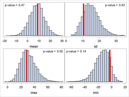
You can plot histograms of each test quantity to visualize the posterior predictive distributions. In addition, you can see where the estimated p-values fall on these densities. Figure 54.18 shows the histograms. To put all four histograms on the same panel, you need to use PROC TEMPLATE to define a new graph template. (See Chapter 21, Statistical Graphics Using ODS. ) The following statements define the template twobytwo:

proc template;
   define statgraph twobytwo;
      begingraph;
         layout lattice / rows=2 columns=2;
            layout overlay / yaxisopts=(display=none)
                             xaxisopts=(label="mean");
               layout gridded / columns=2 border=false
                                autoalign=(topleft topright);
                  entry halign=right "p-value =";
                  entry halign=left eval(strip(put(&pmean, 12.2)));
               endlayout;
               histogram mean / binaxis=false;
               lineparm x=&mean y=0 slope=. /
                        lineattrs=(color=red thickness=5);
            endlayout;
            layout overlay / yaxisopts=(display=none)
                             xaxisopts=(label="sd");
               layout gridded / columns=2 border=false
                                autoalign=(topleft topright);
                  entry halign=right "p-value =";
                  entry halign=left eval(strip(put(&psd, 12.2)));
               endlayout;
               histogram sd / binaxis=false;
               lineparm x=&sd y=0 slope=. /
                        lineattrs=(color=red thickness=5);
            endlayout;
            layout overlay / yaxisopts=(display=none)
                             xaxisopts=(label="max");
               layout gridded / columns=2 border=false
                                autoalign=(topleft topright);
                  entry halign=right "p-value =";
                  entry halign=left eval(strip(put(&pmax, 12.2)));
               endlayout;
               histogram max / binaxis=false;
               lineparm x=&max y=0 slope=. /
                        lineattrs=(color=red thickness=5);
            endlayout;
            layout overlay / yaxisopts=(display=none)
                             xaxisopts=(label="min");
               layout gridded / columns=2 border=false
                                autoalign=(topleft topright);
                  entry halign=right "p-value =";
                  entry halign=left eval(strip(put(&pmin, 12.2)));
               endlayout;
               histogram min / binaxis=false;
               lineparm x=&min y=0 slope=. /
                        lineattrs=(color=red thickness=5);
            endlayout;
         endlayout;
      endgraph;
   end;
run;

You call PROC SGRENDER to create the graph, which is shown in Figure 54.18. (See the SGRENDER procedure in the SAS ODS Graphics: Procedures Guide.) There are no extreme p-values observed; this supports the notion that the predicted results are similar to the actual observations and that the model fits the data.

ods graphics on;
proc sgrender data=pred template=twobytwo;
run;
ods graphics off;

Figure 54.18 Posterior Predictive Distribution Check for the SAT example

Note that the posterior predictive distribution is not the same as the prior predictive distribution. The prior predictive distribution is $\text{[math]}$ , which is also known as the marginal distribution of the data. The prior predictive distribution is an integral of the likelihood function with respect to the prior distribution

$\text{[math]}$

and the distribution is not conditional on observed data.