The MCMC Procedure
-
Overview

-
Getting Started
-
Syntax
-
Details
How PROC MCMC Works Blocking of Parameters Sampling Methods Tuning the Proposal Distribution Conjugate Sampling Initial Values of the Markov Chains Assignments of Parameters Standard Distributions Usage of Multivariate Distributions Specifying a New Distribution Using Density Functions in the Programming Statements Truncation and Censoring Some Useful SAS Functions Matrix Functions in PROC MCMC Create Design Matrix Modeling Joint Likelihood Regenerating Diagnostics Plots Caterpillar Plot Posterior Predictive Distribution Handling of Missing Data Floating Point Errors and Overflows Handling Error Messages Computational Resources Displayed Output ODS Table Names ODS Graphics
-
Examples
Simulating Samples From a Known Density Box-Cox Transformation Logistic Regression Model with a Diffuse Prior Logistic Regression Model with Jeffreys’ Prior Poisson Regression Nonlinear Poisson Regression Models Logistic Regression Random-Effects Model Nonlinear Poisson Regression Random-Effects Model Multivariate Normal Random-Effects Model Change Point Models Exponential and Weibull Survival Analysis Time Independent Cox Model Time Dependent Cox Model Piecewise Exponential Frailty Model Normal Regression with Interval Censoring Constrained Analysis Implement a New Sampling Algorithm Using a Transformation to Improve Mixing Gelman-Rubin Diagnostics
- References
Example 54.6 Nonlinear Poisson Regression Models
This example illustrates how to fit a nonlinear Poisson regression with PROC MCMC. In addition, it shows how you can improve the mixing of the Markov chain by selecting a different proposal distribution or by sampling on the transformed scale of a parameter. This example shows how to analyze count data for calls to a technical support help line in the weeks immediately following a product release. This information could be used to decide upon the allocation of technical support resources for new products. You can model the number of daily calls as a Poisson random variable, with the average number of calls modeled as a nonlinear function of the number of weeks that have elapsed since the product’s release. The data are input into a SAS data set as follows:
title 'Nonlinear Poisson Regression';
data calls;
   input weeks calls @@;
   datalines;
1   0   1   2   2   2   2   1   3   1   3   3
4   5   4   8   5   5   5   9   6  17   6   9
7  24   7  16   8  23   8  27
;
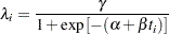
During the first several weeks after a new product is released, the number of questions that technical support receives concerning the product increases in a sigmoidal fashion. The expression for the mean value in the classic Poisson regression involves the log link. There is some theoretical justification for this link, but with MCMC methodologies, you are not constrained to exploring only models that are computationally convenient. The number of calls to technical support tapers off after the initial release, so in this example you can use a logistic-type function to model the mean number of calls received weekly for the time period immediately following the initial release. The mean function  is modeled as follows:
 |
The likelihood for every observation  is
is
 |
Past experience with technical support data for similar products suggests the following prior distributions:
 |
 |
 |
|||
 |
|
 |
|||
 |
|
 |
The following PROC MCMC statements fit this model:
ods graphics on;
proc mcmc data=calls outpost=callout seed=53197 ntu=1000 nmc=20000
propcov=quanew;
ods select TADpanel;
parms alpha -4 beta 1 gamma 2;
prior gamma ~ gamma(3.5, scale=12);
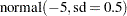
prior alpha ~ normal(-5, sd=0.25);
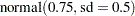
prior beta ~ normal(0.75, sd=0.5);
lambda = gamma*logistic(alpha+beta*weeks);
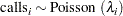
model calls ~ poisson(lambda);
run;
The one PARMS statement defines a block of all parameters and sets their initial values individually. The PRIOR statements specify the informative prior distributions for the three parameters. The assignment statement defines  , the mean number of calls. Instead of using the SAS function LOGISTIC, you can use the following statement to calculate and get the same result:
lambda = gamma / (1 + exp(-(alpha+beta*weeks)));
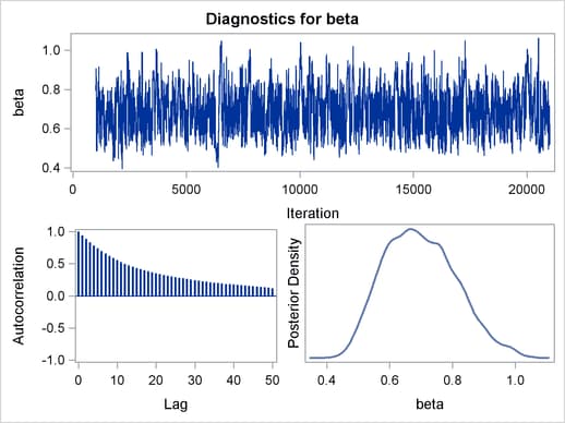
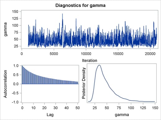
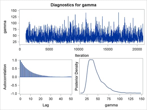
Mixing is not particularly good with this run of PROC MCMC. The ODS SELECT statement displays only the diagnostic graphs while excluding all other output. The graphical output is shown in Output 54.6.1.
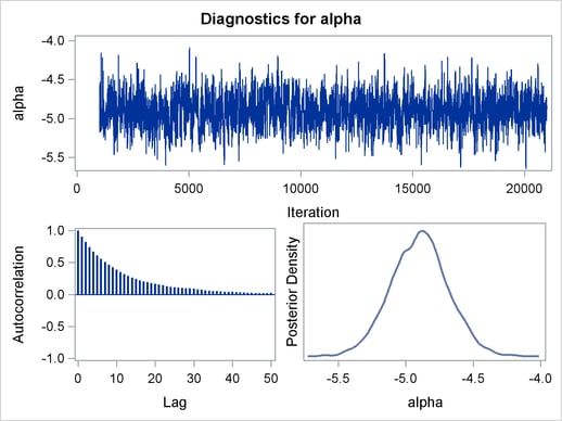
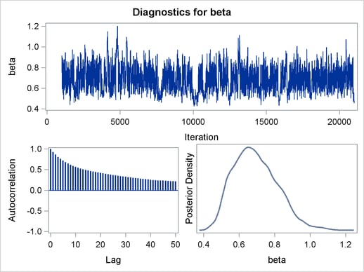
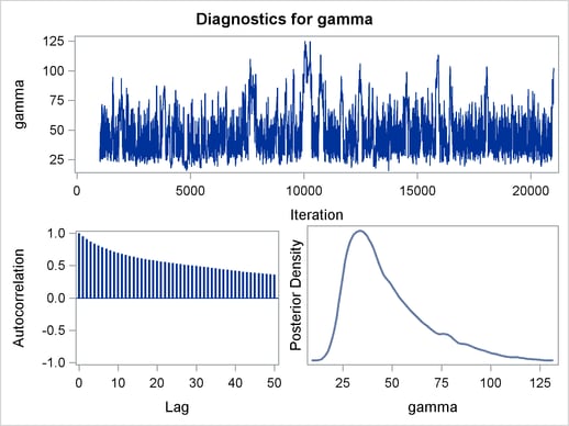
By examining the trace plot of the gamma parameter, you see that the Markov chain sometimes gets stuck in the far right tail and does not travel back to the high density area quickly. This effect can be seen around the simulations number 8000 and 18000. One possible explanation for this is that the random walk Metropolis is taking too small of steps in its proposal; therefore it takes more iterations for the Markov chain to explore the parameter space effectively. The step size in the random walk is controlled by the normal proposal distribution (with a multiplicative scale). A (good) proposal distribution is roughly an approximation to the joint posterior distribution at the mode. The curvature of the normal proposal distribution (the variance) does not take into account the thickness of the tail areas. As a result, a random walk Metropolis with normal proposal can have a hard time exploring distributions that have thick tails. This appears to be the case with the posterior distribution of the parameter gamma. You can improve the mixing by using a thicker-tailed proposal distribution, the t distribution. The PROPDIST= option controls the proposal distribution. PROPDIST=T(3) changes the proposal from a normal distribution to a t distribution with three degrees of freedom.
The following statements run PROC MCMC and produce Output 54.6.2:
proc mcmc data=calls outpost=callout seed=53197 ntu=1000 nmc=20000
          propcov=quanew stats=none propdist=t(3);
   ods select TADpanel;
   parms alpha -4 beta 1 gamma 2;
   prior alpha ~ normal(-5, sd=0.25);
   prior beta  ~ normal(0.75, sd=0.5);
   prior gamma ~ gamma(3.5, scale=12);
   lambda = gamma*logistic(alpha+beta*weeks);
   model calls ~ poisson(lambda);
run;
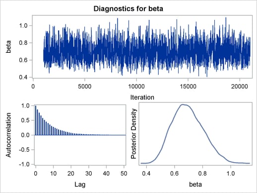
Output 54.6.2 displays the graphical output.
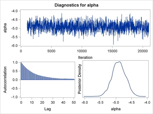
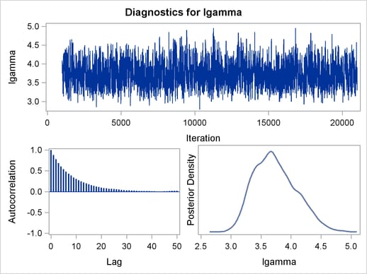
The trace plots are more dense and the ACF plots have faster drop-offs, and you see improved mixing by using a thicker-tailed proposal distribution. If you want to further improve the Markov chain, you can choose to sample the  transformation of the parameter gamma:
 |
The parameter gamma has a positive support. Often in this case, it has right-skewed posterior. By taking the transformation, you can sample on a parameter space that does not have a lower boundary and is more symmetric. This can lead to better mixing.
The following statements produce Output 54.6.4 and Output 54.6.3:
proc mcmc data=calls outpost=callout seed=53197 ntu=1000 nmc=20000
          propcov=quanew propdist=t(3)
          monitor=(alpha beta lgamma gamma);
   ods select PostSummaries PostIntervals TADpanel;
   parms alpha -4 beta 1 lgamma 2;
   prior alpha ~ normal(-5, sd=0.25);
   prior beta  ~ normal(0.75, sd=0.5);
   prior lgamma ~ egamma(3.5, scale=12);
   gamma = exp(lgamma);
   lambda = gamma*logistic(alpha+beta*weeks);
   model calls ~ poisson(lambda);
run;
ods graphics off;
In the PARMS statement, instead of gamma, you have lgamma. Its prior distribution is egamma, as opposed to the gamma distribution. Note that the following two priors are equivalent to each other:
prior lgamma ~ egamma(3.5, scale=12);
prior gamma ~ gamma(3.5, scale=12);
The gamma assignment statement transforms lgamma to gamma. The lambda assignment statement calculates the mean for the Poisson by using the gamma parameter. The MODEL statement specifies a Poisson likelihood for the calls response.
The trace plots and ACF plots in Output 54.6.3 show the best mixing seen so far in this example.

Output 54.6.4 shows the posterior summary statistics of the nonlinear Poisson regression. Note that the lgamma parameter has a more symmetric density than the skewed gamma parameter. The Metropolis algorithm always works better if the target distribution is approximately normal.
| Nonlinear Poisson Regression |
| Posterior Summaries | ||||||
|---|---|---|---|---|---|---|
| Parameter | N | Mean | Standard Deviation |
Percentiles | ||
| 25% | 50% | 75% | ||||
| alpha | 20000 | -4.8907 | 0.2160 | -5.0435 | -4.8872 | -4.7461 |
| beta | 20000 | 0.6957 | 0.1089 | 0.6163 | 0.6881 | 0.7698 |
| lgamma | 20000 | 3.7391 | 0.3487 | 3.4728 | 3.7023 | 3.9696 |
| gamma | 20000 | 44.8136 | 17.0430 | 32.2263 | 40.5415 | 52.9647 |
| Posterior Intervals | |||||
|---|---|---|---|---|---|
| Parameter | Alpha | Equal-Tail Interval | HPD Interval | ||
| alpha | 0.050 | -5.3138 | -4.4667 | -5.3276 | -4.4953 |
| beta | 0.050 | 0.5066 | 0.9253 | 0.4868 | 0.8996 |
| lgamma | 0.050 | 3.1580 | 4.4705 | 3.1222 | 4.4127 |
| gamma | 0.050 | 23.5225 | 87.3972 | 20.9005 | 79.4712 |
This example illustrates that PROC MCMC can fit Bayesian nonlinear models just as easily as Bayesian linear models. More importantly, transformations can sometimes improve the efficiency of the Markov chain, and that is something to always keep in mind. Also see Using a Transformation to Improve Mixing for another example of how transformations can improve mixing of the Markov chains.