The MCMC Procedure
-
Overview

-
Getting Started
-
Syntax
-
Details
How PROC MCMC Works Blocking of Parameters Sampling Methods Tuning the Proposal Distribution Conjugate Sampling Initial Values of the Markov Chains Assignments of Parameters Standard Distributions Usage of Multivariate Distributions Specifying a New Distribution Using Density Functions in the Programming Statements Truncation and Censoring Some Useful SAS Functions Matrix Functions in PROC MCMC Create Design Matrix Modeling Joint Likelihood Regenerating Diagnostics Plots Caterpillar Plot Posterior Predictive Distribution Handling of Missing Data Floating Point Errors and Overflows Handling Error Messages Computational Resources Displayed Output ODS Table Names ODS Graphics
-
Examples
Simulating Samples From a Known Density Box-Cox Transformation Logistic Regression Model with a Diffuse Prior Logistic Regression Model with Jeffreys’ Prior Poisson Regression Nonlinear Poisson Regression Models Logistic Regression Random-Effects Model Nonlinear Poisson Regression Random-Effects Model Multivariate Normal Random-Effects Model Change Point Models Exponential and Weibull Survival Analysis Time Independent Cox Model Time Dependent Cox Model Piecewise Exponential Frailty Model Normal Regression with Interval Censoring Constrained Analysis Implement a New Sampling Algorithm Using a Transformation to Improve Mixing Gelman-Rubin Diagnostics
- References
Example 54.19 Gelman-Rubin Diagnostics
PROC MCMC does not have the Gelman-Rubin test (see the section Gelman and Rubin Diagnostics) as a part of its diagnostics. The Gelman-Rubin diagnostics rely on parallel chains to test whether they all converge to the same posterior distribution. This example demonstrates how you can carry out this convergence test. The regression model from the section Simple Linear Regression is used. The model has three parameters:  and
and  are the regression coefficients, and
  is the variance of the error distribution.
The following statements generate the data set:
title 'Simple Linear Regression, Gelman-Rubin Diagnostics';

data Class;
   input Name $ Height Weight @@;
   datalines;
Alfred  69.0 112.5   Alice  56.5  84.0   Barbara 65.3  98.0
Carol   62.8 102.5   Henry  63.5 102.5   James   57.3  83.0
Jane    59.8  84.5   Janet  62.5 112.5   Jeffrey 62.5  84.0
John    59.0  99.5   Joyce  51.3  50.5   Judy    64.3  90.0
Louise  56.3  77.0   Mary   66.5 112.0   Philip  72.0 150.0
Robert  64.8 128.0   Ronald 67.0 133.0   Thomas  57.5  85.0
William 66.5 112.0
;
To run a Gelman-Rubin diagnostic test, you want to start Markov chains at different places in the parameter space. Suppose that you want to start at  ,
,  , and
, and  ; at
; at  , , and ; and at
  ,
,  , and
, and  . You can put these starting values in the following Init SAS data set:
data init;
   input Chain beta0 beta1 sigma2;
   datalines;
   1   10  -5   1
   2  -15  10  20
   3    0   0  50
;
The following statements run PROC MCMC three times, each with starting values specified in the data set Init:
/* define constants */
%let nchain = 3;
%let nparm = 3;
%let nsim = 50000;
%let var = beta0 beta1 sigma2;

%macro gmcmc;
   %do i=1 %to &nchain;
      data _null_;
         set init;
         if Chain=&i;
         %do j = 1 %to &nparm;
            call symputx("init&j", %scan(&var, &j));
         %end;
         stop;
      run;

      proc mcmc data=class outpost=out&i init=reinit nbi=0 nmc=&nsim
                stats=none seed=7;
         parms beta0 &init1 beta1 &init2;
         parms sigma2 &init3 / n;
         prior beta0 beta1 ~ normal(0, var = 1e6);
         prior sigma2 ~ igamma(3/10, scale = 10/3);
         mu = beta0 + beta1*height;
         model weight ~ normal(mu, var = sigma2);
      run;
   %end;
%mend;

ods listing close;
%gmcmc;
ods listing;
The macro variables nchain, nparm, nsim, and var define the number of chains, the number of parameters, the number of Markov chain simulations, and the parameter names, respectively. The macro GMCMC gets initial values from the data set Init, assigns them to the macro variables init1, init2 and init3, starts the Markov chain at these initial values, and stores the posterior draws to three output data sets: Out1, Out2, and Out3.
In the PROC MCMC statement, the INIT=REINIT option restarts the Markov chain after tuning at the assigned initial values. No burn-in is requested.
You can use the autocall macro GELMAN to calculate the Gelman-Rubin statistics by using the three chains. The GELMAN macro has the following arguments:
%macro gelman(dset, nparm, var, nsim, nc=3, alpha=0.05);
The argument dset is the name of the data set that stores the posterior samples from all the runs, nparm is the number of parameters, var is the name of the parameters, nsim is the number of simulations, nc is the number of chains with a default value of 3, and alpha is the  significant level in the test with a default value of 0.05. This macro creates two data sets: _Gelman_Ests stores the diagnostic estimates and _Gelman_Parms stores the names of the parameters.
The following statements calculate the Gelman-Rubin diagnostics:
data all;
   set out1(in=in1) out2(in=in2) out3(in=in3);
   if in1 then Chain=1;
   if in2 then Chain=2;
   if in3 then Chain=3;
run;

%gelman(all, &nparm, &var, &nsim);

data GelmanRubin(label='Gelman-Rubin Diagnostics');
   merge _Gelman_Parms _Gelman_Ests;
run;

proc print data=GelmanRubin;
run;
The Gelman-Rubin statistics are shown in Output 54.19.1.
| Simple Linear Regression, Gelman-Rubin Diagnostics |
| Obs | Parameter | Between-chain | Within-chain | Estimate | UpperBound |
|---|---|---|---|---|---|
| 1 | beta0 | 5384.76 | 1168.64 | 1.0002 | 1.0001 |
| 2 | beta1 | 1.20 | 0.30 | 1.0002 | 1.0002 |
| 3 | sigma2 | 8034.41 | 2890.00 | 1.0010 | 1.0011 |
The Gelman-Rubin statistics do not reveal any concerns about the convergence or the mixing of the multiple chains. To get a better visual picture of the multiple chains, you can draw overlapping trace plots of these parameters from the three Markov chains runs.
The following statements create Output 54.19.2:
/* plot the trace plots of three Markov chains. */
%macro trace;
   %do i = 1 %to &nparm;
        proc sgplot data=all cycleattrs;
           series x=Iteration y=%scan(&var, &i) / group=Chain;
        run;
   %end;
%mend;
%trace;
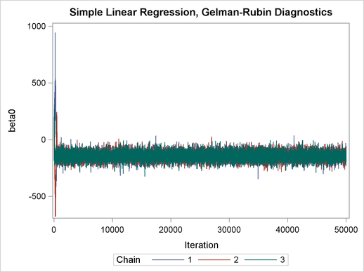
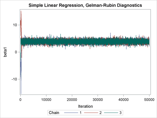
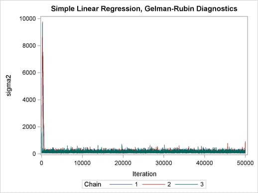
The trace plots show that three chains all eventually converge to the same regions even though they started at very different locations. In addition to the trace plots, you can also plot the potential scale reduction factor (PSRF). See the section Gelman and Rubin Diagnostics for definition and details.
The following statements calculate PSRF for each parameter. They use the GELMAN macro repeatedly and can take a while to run:
/* define sliding window size */
%let nwin = 200;
data PSRF;
run;

%macro PSRF(nsim);
   %do k = 1 %to %sysevalf(&nsim/&nwin, floor);
      %gelman(all, &nparm, &var, nsim=%sysevalf(&k*&nwin));
      data GelmanRubin;
          merge _Gelman_Parms _Gelman_Ests;
      run;

      data PSRF;
         set PSRF GelmanRubin;
      run;
   %end;
%mend PSRF;

options nonotes;
%PSRF(&nsim);
options notes;

data PSRF;
   set PSRF;
   if _n_ = 1 then delete;
run;

proc sort data=PSRF;
   by Parameter;
run;

%macro sepPSRF(nparm=, var=, nsim=);
   %do k = 1 %to &nparm;
       data save&k; set PSRF;
          if _n_ > %sysevalf(&k*&nsim/&nwin, floor) then delete;
          if _n_ < %sysevalf((&k-1)*&nsim/&nwin + 1, floor) then delete;
          Iteration + &nwin;
       run;

       proc sgplot data=save&k(firstobs=10) cycleattrs;
          series x=Iteration y=Estimate;
          series x=Iteration y=upperbound;
          yaxis label="%scan(&var, &k)";
       run;
   %end;
%mend sepPSRF;

%sepPSRF(nparm=&nparm, var=&var, nsim=&nsim);
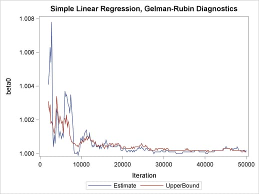
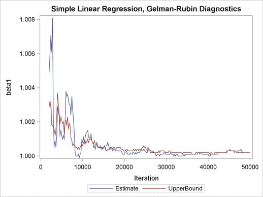
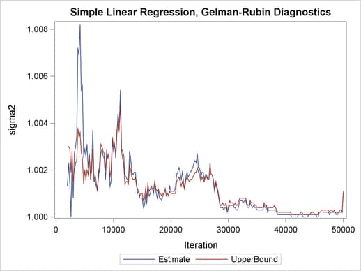
PSRF is the square root of the ratio of the between-chain variance and the within-chain variance. A large PSRF indicates that the between-chain variance is substantially greater than the within-chain variance, so that longer simulation is needed. You want the PSRF to converge to 1 eventually, as it appears to be the case in this simulation study.