The MCMC Procedure
-
Overview

-
Getting Started
-
Syntax
-
Details
How PROC MCMC Works Blocking of Parameters Sampling Methods Tuning the Proposal Distribution Conjugate Sampling Initial Values of the Markov Chains Assignments of Parameters Standard Distributions Usage of Multivariate Distributions Specifying a New Distribution Using Density Functions in the Programming Statements Truncation and Censoring Some Useful SAS Functions Matrix Functions in PROC MCMC Create Design Matrix Modeling Joint Likelihood Regenerating Diagnostics Plots Caterpillar Plot Posterior Predictive Distribution Handling of Missing Data Floating Point Errors and Overflows Handling Error Messages Computational Resources Displayed Output ODS Table Names ODS Graphics
-
Examples
Simulating Samples From a Known Density Box-Cox Transformation Logistic Regression Model with a Diffuse Prior Logistic Regression Model with Jeffreys’ Prior Poisson Regression Nonlinear Poisson Regression Models Logistic Regression Random-Effects Model Nonlinear Poisson Regression Random-Effects Model Multivariate Normal Random-Effects Model Change Point Models Exponential and Weibull Survival Analysis Time Independent Cox Model Time Dependent Cox Model Piecewise Exponential Frailty Model Normal Regression with Interval Censoring Constrained Analysis Implement a New Sampling Algorithm Using a Transformation to Improve Mixing Gelman-Rubin Diagnostics
- References
| Simple Linear Regression |
This section illustrates some basic features of PROC MCMC by using a linear regression model. The model is as follows:
 |
for the observations  .
.
The following statements create a SAS data set with measurements of Height and Weight for a group of children:
title 'Simple Linear Regression';

data Class;
   input Name $ Height Weight @@;
   datalines;
Alfred  69.0 112.5   Alice  56.5  84.0   Barbara 65.3  98.0
Carol   62.8 102.5   Henry  63.5 102.5   James   57.3  83.0
Jane    59.8  84.5   Janet  62.5 112.5   Jeffrey 62.5  84.0
John    59.0  99.5   Joyce  51.3  50.5   Judy    64.3  90.0
Louise  56.3  77.0   Mary   66.5 112.0   Philip  72.0 150.0
Robert  64.8 128.0   Ronald 67.0 133.0   Thomas  57.5  85.0
William 66.5 112.0
;
The equation of interest is as follows:
 |
The observation errors,  , are assumed to be independent and identically distributed with a normal distribution with mean zero and variance
  .
.
 |
The likelihood function for each of the Weight, which is specified in the MODEL statement, is as follows:
 |
where  denotes a conditional probability density and
  is the normal density. There are three parameters in the likelihood:
  ,
,  , and . You use the PARMS statement to indicate that these are the parameters in the model.
Suppose that you want to use the following three prior distributions on each of the parameters:
 |
 |
 |
|||
 |
|
|
|||
 |
|
 |
where  indicates a prior distribution and
  is the density function for the inverse-gamma distribution. The normal priors on and have large variances, expressing your lack of knowledge about the regression coefficients. The priors correspond to an equal-tail
  credible intervals of approximately
  for and . Priors of this type are often called vague or diffuse priors. See the section Prior Distributions for more information. Typically diffuse prior distributions have little influence on the posterior distribution and are appropriate when stronger prior information about the parameters is not available.
A frequently used diffuse prior for the variance parameter is the inverse-gamma distribution. With a shape parameter of  and a scale parameter of
  , this prior corresponds to an equal-tail credible interval of
  , with the mode at
  for . Alternatively, you can use any other positive prior, meaning that the density support is positive on this variance component. For example, you can use the gamma prior.
According to Bayes’ theorem, the likelihood function and prior distributions determine the posterior (joint) distribution of , , and as follows:
 |
 |
 |
You do not need to know the form of the posterior distribution when you use PROC MCMC. PROC MCMC automatically obtains samples from the desired posterior distribution, which is determined by the prior and likelihood you supply.
The following statements fit this linear regression model with diffuse prior information:
ods graphics on;
proc mcmc data=class outpost=classout nmc=10000 thin=2 seed=246810
   mchistory=detailed;
   parms beta0 0 beta1 0;
   parms sigma2 1;
   prior beta0 beta1 ~ normal(mean = 0, var = 1e6);
   prior sigma2 ~ igamma(shape = 3/10, scale = 10/3);
   mu = beta0 + beta1*height;
   model weight ~ n(mu, var = sigma2);
run;
ods graphics off;
When ODS Graphics is enabled, diagnostic plots, such as the trace and autocorrelation function plots of the posterior samples, are displayed. For more information about ODS Graphics, see Chapter 21, Statistical Graphics Using ODS.
The PROC MCMC statement invokes the procedure and specifies the input data set Class. The output data set Classout contains the posterior samples for all of the model parameters. The NMC= option specifies the number of posterior simulation iterations. The THIN= option controls the thinning of the Markov chain and specifies that one of every 2 samples is kept. Thinning is often used to reduce the correlations among posterior sample draws. In this example, 5,000 simulated values are saved in the Classout data set. The SEED= option specifies a seed for the random number generator, which guarantees the reproducibility of the random stream. The MCHISTORY= option produces detailed tuning, burn-in, and sampling history of the Markov chain. For more information about Markov chain sample size, burn-in, and thinning, see the section Burn-in, Thinning, and Markov Chain Samples.
The PARMS statements identify the three parameters in the model: beta0, beta1, and sigma2. Each statement also forms a block of parameters, where the parameters are updated simultaneously in each iteration. In this example, beta0 and beta1 are sampled jointly, conditional on sigma2; and sigma2 is sampled conditional on fixed values of beta0 and beta1. In simple regression models such as this, you expect the parameters beta0 and beta1 to have high posterior correlations, and placing them both in the same block improves the mixing of the chain—that is, the efficiency that the posterior parameter space is explored by the Markov chain. For more information, see the section Blocking of Parameters. The PARMS statements also assign initial values to the parameters (see the section Initial Values of the Markov Chains). The regression parameters are given 0 as their initial values, and the scale parameter sigma2 starts at value 1. If you do not provide initial values, the procedure chooses starting values for every parameter.
The PRIOR statements specify prior distributions for the parameters. The parameters beta0 and beta1 both share the same prior—a normal prior with mean  and variance
  . The parameter sigma2 has an inverse-gamma distribution with a shape parameter of 3/10 and a scale parameter of 10/3. For a list of standard distributions that PROC MCMC supports, see the section Standard Distributions.
The mu assignment statement calculates the expected value of Weight as a linear function of Height. The MODEL statement uses the shorthand notation, n, for the normal distribution to indicate that the response variable, Weight, is normally distributed with parameters mu and sigma2. The functional argument MEAN= in the normal distribution is optional, but you have to indicate whether sigma2 is a variance (VAR=), a standard deviation (SD=), or a precision (PRECISION=) parameter. See Table 54.2 in the section MODEL Statement for distribution specifications.
The distribution parameters can contain expressions. For example, you can write the MODEL statement as follows:
model weight ~ n(beta0 + beta1*height, var = sigma2);
Before you do any posterior inference, it is essential that you examine the convergence of the Markov chain (see the section Assessing Markov Chain Convergence). You cannot make valid inferences if the Markov chain has not converged. A very effective convergence diagnostic tool is the trace plot. Although PROC MCMC produces graphs at the end of the procedure output (see Figure 54.6), you should visually examine the convergence graph first.
The first table that PROC MCMC produces is the "Number of Observations" table, as shown in Figure 54.1. This table lists the number of observations read from the DATA= data set and the number of non-missing observations used in the analysis.
| Simple Linear Regression |
|
|
|---|
The "Parameters" table, shown in Figure 54.2, lists the names of the parameters, the blocking information (see the section Blocking of Parameters), the sampling method used, the starting values (the section Initial Values of the Markov Chains), and the prior distributions. You should check this table to ensure that you have specified the parameters correctly, especially for complicated models.
| Parameters | ||||
|---|---|---|---|---|
| Block | Parameter | Sampling Method |
Initial Value |
Prior Distribution |
| 1 | beta0 | N-Metropolis | 0 | normal(mean = 0, var = 1e6) |
| beta1 | 0 | normal(mean = 0, var = 1e6) | ||
| 2 | sigma2 | Conjugate | 1.0000 | igamma(shape = 3/10, scale = 10/3) |
The first block, which consists of the parameters beta0 and beta1, uses a random walk Metropolis algorithm. The second block, which consists of the parameter sigma2, uses a conjugate updater. The "Tuning History" table, shown in Figure 54.3, shows how the tuning stage progresses for the multivariate random walk Metropolis algorithm. An important aspect of the algorithm is the calibration of the proposal distribution. The tuning of the Markov chain is broken into a number of phases. In each phase, PROC MCMC generates trial samples and automatically modifies the proposal distribution as a result of the acceptance rate (see the section Tuning the Proposal Distribution). In this example, PROC MCMC found an acceptable proposal distribution after two phases, and this distribution is used in both the burn-in and sampling stages of the simulation. Note that the second block contains missing values in “Scale” and “Acceptance Rate” because the conjugate sampler does not use these parameters.
The "Burn-In History" table shows the burn-in phase, and the "Sampling History" table shows the main phase sampling.
| Tuning History | |||
|---|---|---|---|
| Phase | Block | Scale | Acceptance Rate |
| 1 | 1 | 2.3800 | 0.4820 |
| 2 | . | . | |
| 2 | 1 | 3.1636 | 0.3300 |
| 2 | . | . | |
| Burn-In History | ||
|---|---|---|
| Block | Scale | Acceptance Rate |
| 1 | 3.1636 | 0.3280 |
| 2 | . | . |
| Sampling History | ||
|---|---|---|
| Block | Scale | Acceptance Rate |
| 1 | 3.1636 | 0.3377 |
| 2 | . | . |
For each posterior distribution, PROC MCMC also reports summary statistics (posterior means, standard deviations, and quantiles) and interval statistics (95% equal-tail and highest posterior density credible intervals), as shown in Figure 54.4. For more information about posterior statistics, see the section Summary Statistics.
| Simple Linear Regression |
| Posterior Summaries | ||||||
|---|---|---|---|---|---|---|
| Parameter | N | Mean | Standard Deviation |
Percentiles | ||
| 25% | 50% | 75% | ||||
| beta0 | 5000 | -142.8 | 33.4326 | -164.8 | -142.3 | -120.0 |
| beta1 | 5000 | 3.8924 | 0.5333 | 3.5361 | 3.8826 | 4.2395 |
| sigma2 | 5000 | 137.3 | 51.1030 | 101.9 | 127.2 | 161.2 |
| Posterior Intervals | |||||
|---|---|---|---|---|---|
| Parameter | Alpha | Equal-Tail Interval | HPD Interval | ||
| beta0 | 0.050 | -208.9 | -78.7305 | -210.8 | -81.6714 |
| beta1 | 0.050 | 2.8790 | 4.9449 | 2.9056 | 4.9545 |
| sigma2 | 0.050 | 69.1351 | 259.8 | 59.2362 | 236.3 |
By default, PROC MCMC also computes a number of convergence diagnostics to help you determine whether the chain has converged. These are the Monte Carlo standard errors, the autocorrelations at selected lags, the Geweke diagnostics, and the effective sample sizes. These statistics are shown in Figure 54.5. For details and interpretations of these diagnostics, see the section Assessing Markov Chain Convergence.
The "Monte Carlo Standard Errors" table indicates that the standard errors of the mean estimates for each of the parameters are relatively small, with respect to the posterior standard deviations. The values in the "MCSE/SD" column (ratios of the standard errors and the standard deviations) are small, around 0.03. This means that only a fraction of the posterior variability is due to the simulation. The "Autocorrelations of the Posterior Samples" table shows that the autocorrelations among posterior samples reduce quickly and become almost nonexistent after a few lags. The "Geweke Diagnostics" table indicates that no parameter failed the test, and the "Effective Sample Sizes" table reports the number of effective sample sizes of the Markov chain.
| Simple Linear Regression |
| Monte Carlo Standard Errors | |||
|---|---|---|---|
| Parameter | MCSE | Standard Deviation |
MCSE/SD |
| beta0 | 1.0070 | 33.4326 | 0.0301 |
| beta1 | 0.0159 | 0.5333 | 0.0299 |
| sigma2 | 0.9473 | 51.1030 | 0.0185 |
| Posterior Autocorrelations | ||||
|---|---|---|---|---|
| Parameter | Lag 1 | Lag 5 | Lag 10 | Lag 50 |
| beta0 | 0.6177 | 0.1083 | 0.0250 | -0.0007 |
| beta1 | 0.6162 | 0.1052 | 0.0217 | 0.0029 |
| sigma2 | 0.1224 | 0.0216 | 0.0098 | 0.0197 |
| Geweke Diagnostics | ||
|---|---|---|
| Parameter | z | Pr > |z| |
| beta0 | 1.0267 | 0.3046 |
| beta1 | -0.9305 | 0.3521 |
| sigma2 | -0.3578 | 0.7205 |
| Effective Sample Sizes | |||
|---|---|---|---|
| Parameter | ESS | Autocorrelation Time |
Efficiency |
| beta0 | 1102.2 | 4.5366 | 0.2204 |
| beta1 | 1119.0 | 4.4684 | 0.2238 |
| sigma2 | 2910.1 | 1.7182 | 0.5820 |
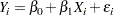
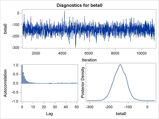
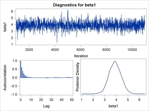
PROC MCMC produces a number of graphs, shown in Figure 54.6, which also aid convergence diagnostic checks. With the trace plots, there are two important aspects to examine. First, you want to check whether the mean of the Markov chain has stabilized and appears constant over the graph. Second, you want to check whether the chain has good mixing and is "dense," in the sense that it quickly traverses the support of the distribution to explore both the tails and the mode areas efficiently. The plots show that the chains appear to have reached their stationary distributions.
Next, you should examine the autocorrelation plots, which indicate the degree of autocorrelation for each of the posterior samples. High correlations usually imply slow mixing. Finally, the kernel density plots estimate the posterior marginal distributions for each parameter.
, and
In regression models such as this, you expect the posterior estimates to be very similar to the maximum likelihood estimators with noninformative priors on the parameters, The REG procedure produces the following fitted model (code not shown):
 |
These are very similar to the means show in Figure 54.4. With PROC MCMC, you can carry out informative analysis that uses specifications to indicate prior knowledge on the parameters. Informative analysis is likely to produce different posterior estimates, which are the result of information from both the likelihood and the prior distributions. Incorporating additional information in the analysis is one major difference between the classical and Bayesian approaches to statistical inference.