The MCMC Procedure
-
Overview

-
Getting Started
-
Syntax
-
Details
How PROC MCMC Works Blocking of Parameters Sampling Methods Tuning the Proposal Distribution Conjugate Sampling Initial Values of the Markov Chains Assignments of Parameters Standard Distributions Usage of Multivariate Distributions Specifying a New Distribution Using Density Functions in the Programming Statements Truncation and Censoring Some Useful SAS Functions Matrix Functions in PROC MCMC Create Design Matrix Modeling Joint Likelihood Regenerating Diagnostics Plots Caterpillar Plot Posterior Predictive Distribution Handling of Missing Data Floating Point Errors and Overflows Handling Error Messages Computational Resources Displayed Output ODS Table Names ODS Graphics
-
Examples
Simulating Samples From a Known Density Box-Cox Transformation Logistic Regression Model with a Diffuse Prior Logistic Regression Model with Jeffreys’ Prior Poisson Regression Nonlinear Poisson Regression Models Logistic Regression Random-Effects Model Nonlinear Poisson Regression Random-Effects Model Multivariate Normal Random-Effects Model Change Point Models Exponential and Weibull Survival Analysis Time Independent Cox Model Time Dependent Cox Model Piecewise Exponential Frailty Model Normal Regression with Interval Censoring Constrained Analysis Implement a New Sampling Algorithm Using a Transformation to Improve Mixing Gelman-Rubin Diagnostics
- References
| Regenerating Diagnostics Plots |
By default, PROC MCMC generates three plots: the trace plot, the autocorrelation plot, and the kernel density plot. Unless ODS Graphics is enabled before calling the procedure, it is hard to generate the same graph afterwards. Directly using the Stat.MCMC.Graphics.TraceAutocorrDensity template is not feasible. The eaiest way to regenerate the same graph is with the %TADPlot autocall macro. The %TADPlot macro requires you to specify an input data set (which typically is the output data set from a previous PROC MCMC call) and a list of variables that you want to plot.
For more information about enabling and disabling ODS Graphics, see the section Enabling and Disabling ODS Graphics in Chapter 21, Statistical Graphics Using ODS.
A simple regression example, with three parameters, is used here for illustrational purposes. For an explanation of the regression model and the data involved, see the section Simple Linear Regression. The following statements generate a SAS data set and fit a regression model:
title 'Regenerating Diagnostics Plots';

data Class;
   input Name $ Height Weight @@;
   datalines;
Alfred  69.0 112.5   Alice  56.5  84.0   Barbara 65.3  98.0
Carol   62.8 102.5   Henry  63.5 102.5   James   57.3  83.0
Jane    59.8  84.5   Janet  62.5 112.5   Jeffrey 62.5  84.0
John    59.0  99.5   Joyce  51.3  50.5   Judy    64.3  90.0
Louise  56.3  77.0   Mary   66.5 112.0   Philip  72.0 150.0
Robert  64.8 128.0   Ronald 67.0 133.0   Thomas  57.5  85.0
William 66.5 112.0
;
ods select none;
proc mcmc data=class nmc=50000 thin=5 outpost=classout seed=246810;
   parms beta0 0 beta1 0;
   parms sigma2 1;
   prior beta0 beta1 ~ normal(0, var = 1e6);
   prior sigma2 ~ igamma(3/10, scale = 10/3);
   mu = beta0 + beta1*height;
   model weight ~ normal(mu, var = sigma2);
run;
ods select all;
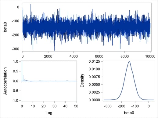
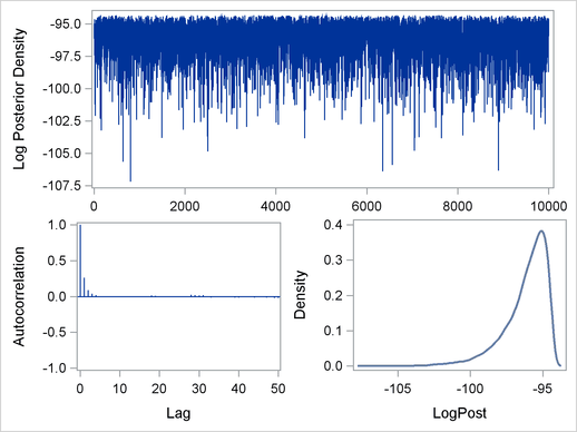
The output data set Classout contains posterior draws for beta0, beta1, and sigma2. It also stores the log of the prior density (LogPrior), log of the likelihood (LogLike), and the log of the posterior density (LogPost). If you want to examine the beta0 and LogPost variable, you can use the following statements to generate the graphs:
ods graphics on;
%tadplot(data=classout, var=beta0 logpost);
ods graphics off;
Figure 54.15 displays the regenerated diagnostics plots for variables beta0 and Logpost from the data set Classout.