The MCMC Procedure
-
Overview

-
Getting Started
-
Syntax
-
Details
How PROC MCMC Works Blocking of Parameters Sampling Methods Tuning the Proposal Distribution Conjugate Sampling Initial Values of the Markov Chains Assignments of Parameters Standard Distributions Usage of Multivariate Distributions Specifying a New Distribution Using Density Functions in the Programming Statements Truncation and Censoring Some Useful SAS Functions Matrix Functions in PROC MCMC Create Design Matrix Modeling Joint Likelihood Regenerating Diagnostics Plots Caterpillar Plot Posterior Predictive Distribution Handling of Missing Data Floating Point Errors and Overflows Handling Error Messages Computational Resources Displayed Output ODS Table Names ODS Graphics
-
Examples
Simulating Samples From a Known Density Box-Cox Transformation Logistic Regression Model with a Diffuse Prior Logistic Regression Model with Jeffreys’ Prior Poisson Regression Nonlinear Poisson Regression Models Logistic Regression Random-Effects Model Nonlinear Poisson Regression Random-Effects Model Multivariate Normal Random-Effects Model Change Point Models Exponential and Weibull Survival Analysis Time Independent Cox Model Time Dependent Cox Model Piecewise Exponential Frailty Model Normal Regression with Interval Censoring Constrained Analysis Implement a New Sampling Algorithm Using a Transformation to Improve Mixing Gelman-Rubin Diagnostics
- References
| Usage of Multivariate Distributions |
The following simple example illustrates the usage of the multivariate distributions in PROC MCMC. Suppose that you are interested in estimating the mean and covariance of multivariate data using this multivariate normal model:
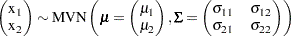 |
where
 |
 |
 |
|||
 |
|
 |
You can use the following independent prior on  and
and  :
:
|
 |
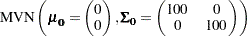 |
|||
|
|
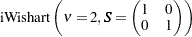 |
The following IML procedure statements simulate 100 random multivariate normal samples:
title 'An Example that Uses Multivariate Distributions';
proc iml;
   N = 100;
   Mean = {1 2};
   Cov =  {2.4 3, 3 8.1};
   call randseed(1);
   x = RANDNORMAL( N, Mean, Cov );

   SampleMean = x[:,];
   n = nrow(x);
   y = x - repeat( SampleMean, n );
   SampleCov = y`*y / (n-1);
   print SampleMean Mean, SampleCov Cov;

   cname = {"x1", "x2"};
   create inputdata from x [colname = cname];
   append from x;
   close inputdata;
   quit;
Figure 54.12 prints the sample mean and covariance of the simulated data, in addition to the true mean and covariance matrix.
| An Example that Uses Multivariate Distributions |
| SampleMean | Mean | ||
|---|---|---|---|
| 0.9987751 | 2.115693 | 1 | 2 |
| SampleCov | Cov | ||
|---|---|---|---|
| 2.8252975 | 3.7190704 | 2.4 | 3 |
| 3.7190704 | 9.2916805 | 3 | 8.1 |
The following PROC MCMC statements estimate the posterior mean and covariance of the multivariate normal data:
proc mcmc data=inputdata seed=17 nmc=3000 diag=none;
   ods select PostSummaries PostIntervals;
   array data[2] x1 x2;
   array mu[2];
   array Sigma[2,2];
   array mu0[2] (0 0);
   array Sigma0[2,2] (100 0 0 100);
   array S[2,2] (1 0 0 1);
   parm mu Sigma;
   prior mu ~ mvn(mu0, Sigma0);
   prior Sigma ~ iwish(2, S);
   model data ~ mvn(mu, Sigma);
   run;
To use the multivariate distribution, you must specify parameters (or random variables in the MODEL statement) in an array form. The first ARRAY statement creates an one-dimensional array data, which contains two numeric variables, x1 and x2, from the input data set. The data variable is your response variable. The subsequent statements defines two array-parameters (mu and Sigma) and three constant array-hyperparameters (mu0, Sigma0, and S). The PARMS statement declares mu and Sigma to be model parameters. The two PRIOR statements specify the multivariate normal and inverse Wishart distributions as the prior for mu and Sigma, respectively. The MODEL statement specifies the multivariate normal likelihood with data as the random variable, mu as the mean, and Sigma as the covariance matrix.
Figure 54.13 lists the estimated posterior mean and covariance matrix.
| Posterior Summaries | ||||||
|---|---|---|---|---|---|---|
| Parameter | N | Mean | Standard Deviation |
Percentiles | ||
| 25% | 50% | 75% | ||||
| mu1 | 3000 | 0.9941 | 0.1763 | 0.8761 | 0.9958 | 1.1136 |
| mu2 | 3000 | 2.1135 | 0.3112 | 1.9075 | 2.1056 | 2.3254 |
| Sigma1 | 3000 | 2.8726 | 0.4084 | 2.5799 | 2.8347 | 3.1205 |
| Sigma2 | 3000 | 3.7573 | 0.6418 | 3.3090 | 3.7057 | 4.1385 |
| Sigma3 | 3000 | 3.7573 | 0.6418 | 3.3090 | 3.7057 | 4.1385 |
| Sigma4 | 3000 | 9.3987 | 1.3224 | 8.4705 | 9.2507 | 10.1946 |
| Posterior Intervals | |||||
|---|---|---|---|---|---|
| Parameter | Alpha | Equal-Tail Interval | HPD Interval | ||
| mu1 | 0.050 | 0.6500 | 1.3356 | 0.6338 | 1.3106 |
| mu2 | 0.050 | 1.5081 | 2.7405 | 1.4939 | 2.7165 |
| Sigma1 | 0.050 | 2.1725 | 3.8034 | 2.1001 | 3.6723 |
| Sigma2 | 0.050 | 2.6659 | 5.2064 | 2.5791 | 5.0223 |
| Sigma3 | 0.050 | 2.6659 | 5.2064 | 2.5791 | 5.0223 |
| Sigma4 | 0.050 | 7.1260 | 12.3763 | 7.0155 | 12.0969 |