The MCMC Procedure

Example 73.22 One-Compartment Model with Pharmacokinetic Data

A popular application of nonlinear mixed models is in the field of pharmacokinetics, which studies how a drug disperses through a living individual. This example considers the theophylline data from Pinheiro and Bates (1995). Serum concentrations of the drug theophylline, which is used to treat respiratory diseases, are measured in 12 subjects over a 25-hour period after oral administration. The data are as follows.

data theoph;
   input subject time conc dose;
   datalines;
 1  0.00  0.74 4.02
 1  0.25  2.84 4.02
 1  0.57  6.57 4.02
 1  1.12 10.50 4.02
 1  2.02  9.66 4.02
 1  3.82  8.58 4.02
 1  5.10  8.36 4.02
 1  7.03  7.47 4.02

   ... more lines ...   

12 24.15  1.17 5.30
;

A commonly used one-compartment model is based on the differential equations

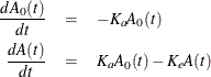
$\begin{eqnarray*} \frac{dA_0(t)}{dt} & =& -K_{a} A_0(t) \\ \frac{dA(t)}{dt} & =& K_{a} A_0(t) - K_{e} A(t) \\ \end{eqnarray*}$

where $K_{a}$ is the absorption rate and $K_{e}$ is the elimination rate.

The initial values are

$\begin{eqnarray*} A_ a(t=0) & =& x \\ A(t=0) & =& 0 \end{eqnarray*}$

where x is the dosage.

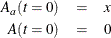
The expected concentration of the substance in the body is computed by dividing the solution to the ODE, $A(t)$ , by Cl, the clearance,

$\begin{eqnarray*} \mu _ i(t) & =& A_ i(t) / \mbox{\Mathtext{Cl}} \\ y_ i(t) & \sim & \mbox{normal}(\mu _ i(t), \sigma ^2) \end{eqnarray*}$

where i is the subject index.

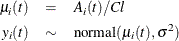
Pinheiro and Bates (1995) consider the following first-order compartment model for these data, where $\log (\mbox{\Mathtext{Cl}})$ and $\log (K_ a)$ are modeled using random effects to account for the patient-to-patient variability:

$\begin{eqnarray*} \mbox{\Mathtext{Cl}}_ i & =& \exp (\beta _1 + b_{i1}) \\ K_{a_ i} & =& \exp (\beta _2 + b_{i2}) \\ K_{e_ i} & =& \exp (\beta _3) \end{eqnarray*}$

Here the $\beta$ s denote fixed-effects parameters and the $b_ i$ s denote random-effects parameters with an unknown covariance matrix.

Although there is an analytical solution to this set of differential equations, this example illustrates the use of a general ODE solver that does not require a closed-form solution. To use the ODE solver, you want to first define the set of differential equations in PROC FCMP and store the objective function, called OneComp, in a user library:

proc fcmp outlib=sasuser.funcs.PK;
   subroutine OneComp(t,y[*],dy[*],ka,ke);
   outargs dy;
   dy[1] = -ka*y[1];
   dy[2] = ka*y[1]-ke*y[2];
   endsub;
run;

The first argument of the OneComp subroutine is the time variable in the differential equation. The second argument is the with-respect-to variable, which can be an array in case a multidimensional problem is required. The third argument is an array that stores the differential equations. This dy argument must also be the OUTARGS variable in the subroutine. The subsequent variables are additional variables, depending on the problem at hand.

In the OneComp subroutine, you can define $K_ a$ and $K_ e$ as functions of $\beta _1$ , $\beta _2$ , and the random-effects parameter $b_2$ . The dy[1] and dy[2] are the differential equation, with dy[1] storing $dA_ a/dt$ and dy[2] storing $dA_ c/dt$ .

The following PROC MCMC statements use the CALL ODE subroutine to solve the set of differential equations defined in OneComp and then use that solution in the construction of the likelihood function:


options cmplib=sasuser.funcs;

proc mcmc data=theoph nmc=10000 seed=27 outpost=theophO diag=none
   nthreads=8;
   ods select PostSumInt;
   array b[2];
   array muB[2] (0 0);
   array cov[2,2];
   array S[2,2] (1 0 0 1);

   array init[2] dose 0;
   array sol[2];

   parms beta1 -3.22 beta2 0.47 beta3 -2.45 ;
   parms cov {0.03 0 0 0.4};
   parms s2y;

   prior beta: ~ normal(0, sd=100);
   prior cov ~ iwish(2, S);
   prior s2y  ~ igamma(shape=3, scale=2);

   random b ~ mvn(muB, cov) subject=subject;
   cl   = exp(beta1 + b1);
   ka   = exp(beta2 + b2);
   ke   = exp(beta3);
   v    = cl/ke;
   call ode('OneComp',sol,init,0,time,ka,ke);
   mu   = (sol[2]/v);
   model conc ~ normal(mu,var=s2y);
run;

The INIT array stores the initial values of the two differential equations, with $A_ a(t=0)=\mbox{\Variable{dose}}$ and $A(t=0)=0$ . The array is used as an input argument to the CALL ODE subroutine.

The RANDOM statement specifies two-dimensional random effects, b, with a multivariate normal prior. The first random effect, b1, enters the model through the clearance variable, cl. The second random effect, b2, is part of the differential equations. The CALL ODE subroutine solves the OneComp set of differential equations and returns the solution to the SOL array. The second array element, SOL[2], is the solution to $A_ i(t)$ for every subject i at every time t.

Posterior summary statistics are reported in Output 73.22.1.

Output 73.22.1: Posterior Summary Statistics

The MCMC Procedure

Posterior Summaries and Intervals
Parameter	N	Mean	Standard Deviation	95% HPD Interval
beta1	10000	-3.2073	0.0836	-3.3768	-3.0429
beta2	10000	0.4375	0.1860	0.1112	0.7671
beta3	10000	-2.4608	0.0547	-2.5642	-2.3576
cov1	10000	0.1312	0.0637	0.0429	0.2507
cov2	10000	-0.00248	0.0919	-0.1876	0.1793
cov3	10000	-0.00248	0.0919	-0.1876	0.1793
cov4	10000	0.6155	0.3175	0.1897	1.2190
s2y	10000	0.5246	0.0719	0.3954	0.6714

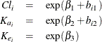
In this problem, the closed-form solution of the ODE is known:

$C_{it} = \frac{D k_{e_ i} k_{a_ i}}{Cl_ i(k_{a_ i} - k_{e_ i})} [\exp (-k_{e_ i} t) - \exp (-k_{a_ i} t)] + e_{it}$

You can manually enter the equation in PROC MCMC and use the following program to fit the same model:

proc mcmc data=theoph nmc=10000 seed=22 outpost=theophC;
   array b[2];

   array mu[2] (0 0);
   array cov[2,2];
   array S[2,2] (1 0 0 1);

   parms beta1 -3.22 beta2 0.47 beta3 -2.45 ;
   parms cov {0.03 0 0 0.4};
   parms s2y;

   prior beta: ~ normal(0, sd=100);
   prior cov ~ iwish(2, S);
   prior s2y  ~ igamma(shape=3, scale=2);

   random b ~ mvn(mu, cov) subject=subject;
   cl   = exp(beta1 + b1);
   ka   = exp(beta2 + b2);
   ke   = exp(beta3);
   pred = dose*ke*ka*(exp(-ke*time)-exp(-ka*time))/cl/(ka-ke);
   model conc ~ normal(pred,var=s2y);
run;

Because this program makes it unnecessary to numerically solve the ODE at every observation and every iteration, it runs much faster than the program that uses the CALL ODE subroutine. But few pharmacokinetic models have known solutions that enable you to do that.