The MCMC Procedure
-
Overview

-
Getting Started
-
Syntax
-
DetailsHow PROC MCMC WorksBlocking of ParametersSampling MethodsTuning the Proposal DistributionDirect SamplingConjugate SamplingInitial Values of the Markov ChainsAssignments of ParametersStandard DistributionsUsage of Multivariate DistributionsSpecifying a New DistributionUsing Density Functions in the Programming StatementsTruncation and CensoringSome Useful SAS FunctionsMatrix Functions in PROC MCMCCreate Design MatrixModeling Joint LikelihoodAccess Lag and Lead VariablesCALL ODE and CALL QUAD SubroutinesRegenerating Diagnostics PlotsCaterpillar PlotAutocall Macros for PostprocessingGamma and Inverse-Gamma DistributionsPosterior Predictive DistributionHandling of Missing DataFunctions of Random-Effects ParametersFloating Point Errors and OverflowsHandling Error MessagesComputational ResourcesDisplayed OutputODS Table NamesODS Graphics
-
ExamplesSimulating Samples From a Known DensityBox-Cox TransformationLogistic Regression Model with a Diffuse PriorLogistic Regression Model with Jeffreys’ PriorPoisson RegressionNonlinear Poisson Regression ModelsLogistic Regression Random-Effects ModelNonlinear Poisson Regression Multilevel Random-Effects ModelMultivariate Normal Random-Effects ModelMissing at Random AnalysisNonignorably Missing Data (MNAR) AnalysisChange Point ModelsExponential and Weibull Survival AnalysisTime Independent Cox ModelTime Dependent Cox ModelPiecewise Exponential Frailty ModelNormal Regression with Interval CensoringConstrained AnalysisImplement a New Sampling AlgorithmUsing a Transformation to Improve MixingGelman-Rubin DiagnosticsOne-Compartment Model with Pharmacokinetic Data
- References
Access Lag and Lead Variables
There are two types of random variables in PROC MCMC that are indexed: the response (MODEL
statement) is indexed by observations, and the random effect (RANDOM
statement) is indexed by the SUBJECT=
option variable. As the procedure steps through the input data set, the response or the random-effects symbols are filled
with values of the current observation or the random-effects parameters in the current subject. Often you might want to access
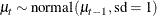
lag or lead variables across an index. For example, the likelihood function for  can depend on
  in an autoregressive model, or the prior distribution for
  can depend on
  , where
  , in a dynamic linear model. In these situations, you can use the following rules to construct symbols to access values from
other observations or subjects:
, in a dynamic linear model. In these situations, you can use the following rules to construct symbols to access values from
other observations or subjects:
-
rv.Li: the ith lag of the variablerv. This looks back to the past. -
rv.Ni: the ith lead of the variablerv. This looks forward to the future.
The construction is allowed for random variables that are associated with an index, either a response variable or a random-effects variable. You concatenate the variable name, a dot, either the letter L (for “lag”) or the letter N (for “next”), and a lag or a lead number. PROC MCMC resolves these variables according to the indices that are associated with the random variable, with respect to the current observation.
For example, the following RANDOM statement specifies a first-order Markov dependence in the random effect mu that is indexed by the subject variable time:
random mu ~ normal(mu.l1,sd=1) subject=time;
This corresponds to the prior
At each observation, PROC MCMC fills in the symbol mu with the random-effects parameter  that belongs to the current cluster t. To fill in the symbol
 mu.l1, the procedure looks back and finds a lag-1 random-effects parameter,  , from the last cluster t-1. As the procedure moves forward in the input data set, these two symbols are constantly updated, as appropriate.
When the index is out of range, such as t–1 when t is 1, PROC MCMC fills in the missing state from the ICOND= option in either the MODEL or RANDOM statement. The following example illustrates how PROC MCMC fills in the values of these lag and lead variables as it steps through the data set.
Assume that the random effect mu has five levels, indexed by 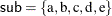 . The model contains two lag variables and one lead variable (
mu.l1, mu.l2, and mu.n2):
mn = (mu.l1 + mu.l2 + mu.n2) / 3
random mu ~ normal(mn, sd=1) subject=time icond=(alpha beta gamma kappa);
In this setup, instead of a list of five random-effects parameters that the variable mu can be assigned values to, there is now a list of nine variables for the variables mu, mu.l1, mu.l2, and mu.n2. The list lines up in the following order:
![\[ \mbox{\Variable{alpha}}, \mbox{\Variable{beta}}, \mu _{\mbox{a}}, \mu _{\mbox{b}}, \mu _{\mbox{c}}, \mu _{\mbox{d}}, \mu _{\mbox{e}}, \mbox{\Variable{gamma}}, \mbox{\Variable{kappa}} \]](images/statug_mcmc0532.png)
PROC MCMC finds relevant symbol values according to this list, as the procedure steps through different subject cluster. The process is illustrated in Table 73.45.
Table 73.45: Processing Lag and Lead Variables
|
|
|
|
|
|
|
a |
|
|
|
|
|
b |
|
|
|
|
|
c |
|
|
|
|
|
d |
|
|
|
|
|
e |
|
|
|
|
For observations in cluster a, PROC MCMC sets the random-effects variable mu to  , looks back two lags and fills in
 mu.l2 with alpha, looks back one lag and fills in mu.l1 with beta, and looks forward two leads and fills in mu.n2 with  . As the procedure moves to observations in cluster b,
 mu becomes  ,
, mu.l2 becomes beta, mu.l1 becomes , and mu.n2 becomes  . For observations in the last cluster, cluster e,
 mu becomes  ,
, mu.l2 becomes , mu.l1 becomes , and mu.n2 is filled with kappa.
The following example fits a simple first-order dynamic linear model, in which the data set contains a time index and the response variable y:
data dlm;
   input time y;
   datalines;
1   1.353412529
2   4.840739953
3   1.604892523
4   6.8947921
5   3.509644288
6   4.020173553
7   3.842884451
8   4.49057276
9   2.204570502
10   4.007351323
11   2.005515044
12   2.781756057
;
You can fit the following model to the data:
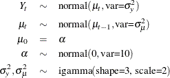
The following PROC MCMC statements estimate parameters from this dynamic linear model:
proc mcmc data=dlm outpost=dlmO nmc=20000 seed=23;
   ods select PostSumInt;
   parms alpha 0;
   parms var_y 1 var_mu 1;
   prior alpha ~ n(0, sd=10);
   prior var_y var_mu ~ igamma(shape=3, scale=2);
   random mu ~ n(mu.l1,var=var_mu) s=time icond=(alpha) monitor=(mu);
   model y~n(mu, var=var_y);
run;
The key component is the mu.l1 specification in the RANDOM
statement, where the prior for mu depends on its lag-1 value. The ICOND=
option specifies the initial condition of mu and assigns it to be alpha, which is a parameter in the model.
Figure 73.16 lists the estimated posterior statistics for the parameters.
Figure 73.16: Posterior Summary Statistics of the Dynamic Linear Model
| Posterior Summaries and Intervals | |||||
|---|---|---|---|---|---|
| Parameter | N | Mean | Standard Deviation |
95% HPD Interval | |
| alpha | 20000 | 2.6498 | 1.2924 | -0.0555 | 5.0366 |
| var_y | 20000 | 1.7400 | 0.8337 | 0.5651 | 3.3498 |
| var_mu | 20000 | 0.8299 | 0.5720 | 0.2109 | 1.9582 |
| mu_1 | 20000 | 2.6899 | 0.9253 | 0.8380 | 4.5390 |
| mu_2 | 20000 | 3.4175 | 0.7622 | 1.9336 | 4.9541 |
| mu_3 | 20000 | 3.3820 | 0.7431 | 1.8543 | 4.7950 |
| mu_4 | 20000 | 4.3364 | 0.8297 | 2.7406 | 6.0198 |
| mu_5 | 20000 | 3.9308 | 0.7194 | 2.4967 | 5.3248 |
| mu_6 | 20000 | 3.8642 | 0.7348 | 2.4117 | 5.3832 |
| mu_7 | 20000 | 3.7716 | 0.7399 | 2.3019 | 5.1525 |
| mu_8 | 20000 | 3.6754 | 0.7316 | 2.1683 | 5.0342 |
| mu_9 | 20000 | 3.1796 | 0.7209 | 1.7485 | 4.6257 |
| mu_10 | 20000 | 3.2237 | 0.7355 | 1.7802 | 4.6253 |
| mu_11 | 20000 | 2.8074 | 0.7839 | 1.2985 | 4.3701 |
| mu_12 | 20000 | 2.8006 | 0.8758 | 1.1286 | 4.5473 |