The MCMC Procedure

Example 73.17 Normal Regression with Interval Censoring

You can use PROC MCMC to fit failure time data that can be right, left, or interval censored. To illustrate, a normal regression model is used in this example.

Assume that you have the following simple regression model with no covariates:

$\mb{y} = \mu + \sigma \bepsilon$

where $\mb{y}$ is a vector of response values (the failure times), $\mu$ is the grand mean, $\sigma$ is an unknown scale parameter, and $\bepsilon$ are errors from the standard normal distribution. Instead of observing $y_ i$ directly, you only observe a truncated value $t_ i$ . If the true $y_ i$ occurs after the censored time $t_ i$ , it is called right censoring. If $y_ i$ occurs before the censored time, it is called left censoring. A failure time $y_ i$ can be censored at both ends, and this is called interval censoring. The likelihood for $y_ i$ is as follows:

$p(y_ i | \mu ) = \left\{ \begin{array}{ll} \phi (y_ i | \mu , \sigma ) & \mbox{if } y_ i \mbox{ is uncensored} \\ S(t_{l,i} | \mu ) & \mbox{if } y_ i \mbox{ is right censored by } t_{l,i}\\ 1 - S(t_{r,i}|\mu ) & \mbox{if } y_ i \mbox{ is left censored by } t_{r,i} \\ S(t_{l,i} | \mu ) - S(t_{r,i}|\mu ) & \mbox{if } y_ i \mbox{ is interval censored by } t_{l,i} \mbox{ and } t_{r,i} \end{array} \right.$

where $S(\cdot )$ is the survival function, $S(t) = \mbox{Pr}(T > t)$ .

Gentleman and Geyer (1994) uses the following data on cosmetic deterioration for early breast cancer patients treated with radiotherapy:

title 'Normal Regression with Interval Censoring';
data cosmetic;
   label tl = 'Time to Event (Months)';
   input tl tr @@;
   datalines;
45  .   6 10   .  7  46  .  46  .   7 16  17  .   7 14
37 44   .  8   4 11  15  .  11 15  22  .  46  .  46  .
25 37  46  .  26 40  46  .  27 34  36 44  46  .  36 48
37  .  40  .  17 25  46  .  11 18  38  .   5 12  37  .
 .  5  18  .  24  .  36  .   5 11  19 35  17 25  24  .
32  .  33  .  19 26  37  .  34  .  36  .
;

The data consist of time interval endpoints (in months). Nonmissing equal endpoints (tl = tr) indicates noncensoring; a nonmissing lower endpoint (tl $\neq$ .) and a missing upper endpoint (tr = .) indicates right censoring; a missing lower endpoint (tl = .) and a nonmissing upper endpoint (tr $\neq$ .) indicates left censoring; and nonmissing unequal endpoints (tl $\neq$ tr) indicates interval censoring.

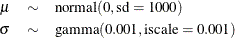
With this data set, you can consider using proper but diffuse priors on both $\mu$ and $\sigma$ , for example:

$\begin{eqnarray*} \mu & \sim & \mbox{normal}(0, \mbox{sd}=1000) \\ \sigma & \sim & \mbox{gamma}(0.001, \mbox{iscale} = 0.001) \end{eqnarray*}$

The following SAS statements fit an interval censoring model and generate Output 73.17.1:

proc mcmc data=cosmetic outpost=postout seed=1 nmc=20000 missing=AC;
   ods select PostSumInt;
   parms mu 60 sigma 50;

   prior mu ~ normal(0, sd=1000);
   prior sigma ~ gamma(shape=0.001,iscale=0.001);

   if (tl^=. and tr^=. and tl=tr) then
      llike = logpdf('normal',tr,mu,sigma);
   else if (tl^=. and tr=.) then
      llike = logsdf('normal',tl,mu,sigma);
   else if (tl=. and tr^=.) then
      llike = logcdf('normal',tr,mu,sigma);
   else
      llike = log(sdf('normal',tl,mu,sigma) -
         sdf('normal',tr,mu,sigma));

   model general(llike);
run;

Because there are missing cells in the input data, you want to use the MISSING=AC option so that PROC MCMC does not delete any observations that contain missing values. The IF-ELSE statements distinguish different censoring cases for $y_ i$ , according to the likelihood. The SAS functions LOGCDF, LOGSDF, LOGPDF, and SDF are useful here. The MODEL statement assigns llike as the log likelihood to the response. The Markov chain appears to have converged in this example (evidence not shown here), and the posterior estimates are shown in Output 73.17.1.

Output 73.17.1: Interval Censoring

Normal Regression with Interval Censoring

The MCMC Procedure

Posterior Summaries and Intervals
Parameter	N	Mean	Standard Deviation	95% HPD Interval
mu	20000	41.7807	5.7882	31.3604	53.6115
sigma	20000	29.1122	6.0503	19.4041	41.6742