The MCMC Procedure
-
Overview

-
Getting Started
-
Syntax
-
DetailsHow PROC MCMC WorksBlocking of ParametersSampling MethodsTuning the Proposal DistributionDirect SamplingConjugate SamplingInitial Values of the Markov ChainsAssignments of ParametersStandard DistributionsUsage of Multivariate DistributionsSpecifying a New DistributionUsing Density Functions in the Programming StatementsTruncation and CensoringSome Useful SAS FunctionsMatrix Functions in PROC MCMCCreate Design MatrixModeling Joint LikelihoodAccess Lag and Lead VariablesCALL ODE and CALL QUAD SubroutinesRegenerating Diagnostics PlotsCaterpillar PlotAutocall Macros for PostprocessingGamma and Inverse-Gamma DistributionsPosterior Predictive DistributionHandling of Missing DataFunctions of Random-Effects ParametersFloating Point Errors and OverflowsHandling Error MessagesComputational ResourcesDisplayed OutputODS Table NamesODS Graphics
-
ExamplesSimulating Samples From a Known DensityBox-Cox TransformationLogistic Regression Model with a Diffuse PriorLogistic Regression Model with Jeffreys’ PriorPoisson RegressionNonlinear Poisson Regression ModelsLogistic Regression Random-Effects ModelNonlinear Poisson Regression Multilevel Random-Effects ModelMultivariate Normal Random-Effects ModelMissing at Random AnalysisNonignorably Missing Data (MNAR) AnalysisChange Point ModelsExponential and Weibull Survival AnalysisTime Independent Cox ModelTime Dependent Cox ModelPiecewise Exponential Frailty ModelNormal Regression with Interval CensoringConstrained AnalysisImplement a New Sampling AlgorithmUsing a Transformation to Improve MixingGelman-Rubin DiagnosticsOne-Compartment Model with Pharmacokinetic Data
- References
CALL ODE and CALL QUAD Subroutines
The CALL ODE subroutine numerically solves a set of first-order ordinary differential equations (ODEs), including piecewise differential equations. The CALL QUAD subroutine calculates multidimensional integrand. You can use them as programming statements in PROC MCMC. These subroutines require that you define an objective function, for either a set of simultaneous differential equations or an integrand function, by using PROC FCMP (see the FCMP procedure in the Base SAS Procedures Guide) and call these subroutines in PROC MCMC.
CALL ODE
The CALL ODE subroutine performs numerical integration of first-order vector differential equations of the form  over the subinterval
 ![$t \in [t_ i,t_ f]$](images/statug_mcmc0540.png) with the initial values
with the initial values  . The subroutine can also be used to solve piecewise differential equations.
You specify the CALL ODE subroutine in PROC MCMC by using the following syntax:
CALL ODE("DeqFun", Soln, Init, ti, tf, G1, G2, ... , Gk <, ode_opt>);
DeqFun: the name of the PROC FCMP subroutine of a set of simultaneous set of ordinary differential equations,
Soln: an argument that contains solutions. Soln can be a numeric variable or an array. If it is an array, then the size of the array determines the dimension of the problem.
Otherwise, the dimension of the problem is one.
Init: initial values of the variable y. Init can be either a numeric variable or an array. The dimension must match that of Soln.
ti: initial time value of the subinterval t
tf: final time value of the subinterval t
Gi: input arguments in the DeqFun subroutine
ode_opt: subroutine options. ode_opt is a positional array of size 4, with the following definition:
-
ode_opt[1]: convergence accuracy. The default value is 1E–8. -
ode_opt[2]: minimum allowable step size in the integration process. The default value is 1E–12. -
ode_opt[3]: maximum allowable step size in the integration process. The default value is the largest double-precision floating-point number. -
ode_opt[4]: initial step size to start the integration process. The default value is 1E–5.
To specify the DeqFun subroutine by using PROC FCMP, use the following statements:
proc fcmp outlib=sasuser.funcs.ODE;
   subroutine DeqFun(t,y[*],dy[*], A1,A2,...,Ak);
   outargs dy;
   dy[1] = -A1*y[1];
   dy[2] = A2*y[1]-Ak-1*y[2];
   ...
   dy[n] = t*y[n] + Ak;
   endsub;
run;
The OUTLIB= option specifies an output data set to which the compiled subroutine is written. The first three arguments of
the DeqFun subroutine must be (1) the time variable t, (2) the with-respect-to variable y, which can be an array, and (3) the differential equation function variable dy, which can also be an array. The remaining optional input arguments are variables that are required in the construction of
the differential equations. You must declare variable dy as the updated variable in the OUTARGS statement.
To include the DeqFun in your PROC MCMC program, you must specify the SAS data set that contains the compiler subroutine:
options cmplib=sasuser.funcs;
See One-Compartment Model with Pharmacokinetic Data for an example of fitting a pharmacokinetic model by using the CALL ODE subroutine.
The CALL ODE subroutine uses the polyalgorithm of Byrne and Hindmarsh (1975) to provide a numerical solution for the set of ordinary differential equations. Note that you can model any n-order differential equation as a system of first-order differential equations.
Piecewise Differential Equations
Suppose you have a system of piecewise ODEs of the following form:
![\[ \frac{d\mb{y}}{dt} = \left\{ \begin{array}{ll} f_1(t, \mb{y}(t)) & t_1 \leq t < t_2 \\ f_2(t, \mb{y}(t)) & t_2 \leq t < t_3 \\ \vdots & \vdots \\ f_{m-1}(t, \mb{y}(t)) & t_{m-1} \leq t < t_{m} \\ f_ m(t, \mb{y}(t)) & t_ m \leq t \\ \end{array} \right. \]](images/statug_mcmc0542.png)
The system of equations is defined over m intervals (![$t \in [t_ i, t_ f]$](images/statug_mcmc0543.png) ) with initial values
) with initial values  for
for  . The variable
  can be a vector. The CALL ODE subroutine solves the system of piecewise ODEs in each semiclosed interval
  for
for  .
.
The CALL ODE subroutine differentiates between a regular ODE problem and a piecewise ODE problem based on the dimension of
the second input argument to the subroutine. That is the Soln argument, which stores the solutions to the ODEs. If Soln is either a numeric variable or a one-dimensional array, the CALL ODE subroutine treats the problem as a regular ODE problem;
if Soln is a two-dimensional array, the CALL ODE subroutine treats it as a piecewise ODE problem and solves accordingly.
You specify the CALL ODE subroutine in PROC MCMC to solve piecewise ODEs by using the following syntax:
CALL ODE("DeqFun", Soln, ., ti, tf, G1, G2, ... , Gk,
         ode_grid, "InitFun", H1, H2, ..., Hl <, ode_opt>);
DeqFun: the name of the PROC FCMP subroutine of a system of ODEs
Soln: an argument that contains solutions. Soln must be an m (number of intervals)  n (number of equations) array. Upon completion, the CALL ODE subroutine fills in the last row of the
 Soln array (![$\mbox{\Variable{Soln}}[m,1], \ldots , \mbox{\Variable{Soln}}[m,n]$](images/statug_mcmc0550.png) ) with the final solutions.
) with the final solutions.
. (period): the third positional argument takes a missing value, or a period (.). In a regular ODE problem, the third argument
is reserved for initial values, which are fixed per solution. In a piecewise problem, initial values can depend on solutions
to previous set of ODEs, and they are set through a separate PROC FCMP subroutine (see description of InitFun).
ti: initial time value of the subinterval t
tf: final time value of the subinterval t
Gi: input arguments in the DeqFun subroutine
ode_grid: numerical array that stores the interval boundaries. You must use the keyword ode_grid for this array, and the array should be placed after all the Gi variables. Elements in ode_grid must be sorted in ascending order. The dimension of this array should be m, the number of rows in Soln.
InitFun: the name of the PROC FCMP subroutine that specifies the initial values of the ODEs at different intervals. The subroutine
requires an output array argument that should be filled with the required initial values for each interval. The InitFun subroutine should come after the ode_grid variable.
Hi: input arguments in the InitFun subroutine
ode_opt: subroutine options
The following example statements construct a two-interval piecewise ODE in the DeqFun subroutine, set initial values in the InitFun subroutine, and call the general ODE solver in PROC MCMC:
proc fcmp outlib=sasuser.funcs.ODE;
   subroutine DeqFun(t,y[*],dy[*],t1,beta,alpha);
   outargs dy;
   if (t <= t1) then do;
       dy[1] = -y[1];
       dy[2] = beta * y[1] - y[2];
       dy[3] = - y[3];
   end; else do;
       dy[1] = 0;
       dy[2] = alpha * y[1] + y[2];
       dy[3] = alpha * y[3] * y[3];
   end;
   endsub;
run;

proc fcmp outlib=sasuser.funcs.ODE;
   subroutine InitFun(init[*,*],d,Soln[*,*]);
   outargs init;
   init[1,1] = d;
   init[1,2] = d;
   init[1,3] = d;
   init[2,1] = Soln[1,1];
   init[2,2] = Soln[1,2];
   init[2,3] = Soln[1,3];
   endsub;
run;

options cmplib=sasuser.funcs;

proc mcmc ...;
   array Soln[2, 3];
   array ode_grid[2];

   ode_grid[1]=0;
   ode_grid[2]=ti;
   call ode("DeqFun", Soln, ., 0, tf, ti, beta, alpha,
            ode_grid, "InitFun", dose, Soln);
   ...;
run;
The DeqFun subroutine specifies three differential equations in two intervals,  and
and  . The
. The InitFun subroutine specifies the initial values for the first set of equations as d (an input variable) and specifies the initial values for the second set of equations as solutions to the first set of equations.
In the PROC MCMC statements, Soln is an array of size 2 3. The ode_grid array has two elements: the first element is the lower bound (0 in this case), and the second element is ti (for example, a data set variable). The DeqFun and InitFun subroutines are passed to the ODE solver. Three variables (ti, beta, and alpha) are input arguments to the DeqFun subroutine. Two variables (dose and Soln) are input arguments to the InitFun subroutine. The solution array, Soln, is passed to the InitFun subroutine and enables the ODE solver to use solutions to the first set of ODEs as the initial values for the second set.
The CALL ODE subroutine fills the second row of the Soln array (Soln[2,1], Soln[2,2], and Soln[2,3]) with the final solution to the entire system of the ODEs upon completion.
CALL QUAD
The CALL QUAD subroutine is a numerical integrator that performs the integration in a twofold fashion based on the dimension of the problem. In a unidimensional problem, the subroutine uses the adaptive Romberg type of integration techniques; in a multidimensional problem, it uses the Laplace approximation. You specify the CALL QUAD subroutine syntax in PROC MCMC by using the following syntax:
CALL QUAD("IntFun",Res, LL, UL, G1, G2, ... , Gk <, quad_init> <, quad_opt>);
IntFun: the name of the PROC FCMP subroutine of an integrand function
Res: contains the approximated integral value
LL: lower limit of the integral. LL must be an array if the problem is multidimensional.
UL: upper limit of the integral. UL must be an array if the problem is multidimensional.
Gi: input arguments in the IntFun subroutine
quad_init: starting values that are used in optimizing the IntFun function in Laplace approximation. This optional array is applicable only in a multidimensional problem, and you must use
the keyword quad_init for this array. By default, the optimization starts at the average values of LL and UL. When you use the variable quad_init, it must precede the integration option array quad_opt.
quad_opt: integration options. You must use the keyword quad_opt for this array. For a unidimensional integration problem, quad_opt must be a positional array of size 4:
-
quad_opt[1]: relative accuracy. The default value is 1E–7. -
quad_opt[2]: the approximate location of a maximum of the integrand. The default value is the centered location between theLLandULlimits. -
quad_opt[3]: approximate estimate of any scale in the integrand along the independent variables. The default value is 1. -
quad_opt[4]: the number of refinements allowed in order to achieve the required accuracy
In a multidimensional integration problem, quad_opt is a positional array of size 2:
-
quad_opt[1]: relative accuracy. The default value is 1E–7.
-
quad_opt[2]: optimization technique:
-
1: Quasi-Newton
-
2: Newton-Raphson
-
3: Newton-Raphson with ridging
-
4: Nelder-Mead simplex method
-
To specify the subroutine IntFun in PROC FCMP, you can use the following example:
proc fcmp outlib=sasuser.funcs.QUAD;
   subroutine IntFun(y[*],fy,pi);
   outargs fy;
   fy = (exp(-(y[1]*y[1]+y[2]*y[2])/2))/(2*pi);
   endsub;
run;
The first argument to IntFun must be the with-respect-to vector in the integral. The variable y can be a scalar or an array, depending on your problem. The second argument must be the variable that contains the integrand
value, which should be declared as the updated variable in the OUTARGS statement. The remaining input arguments are optional
variables, if needed in constructing the integrand function.
To include the IntFun subroutine in your PROC MCMC program, you must specify the SAS data set that contains the compiler subroutine:
options cmplib=sasuser.funcs;

proc mcmc ...;
   array LL[2] (-100 -100);
   array UL[2] ( 100  100);

   call quad("IntFun", Res, LL, UL, pi);
   ...;
run;
In the PROC MCMC statements, LL and UL are arrays that contain the lower and upper limits of the integral. The variable pi is an input argument to the IntFun subroutine. The solution is stored in Res.
In case of one-dimensional integration, the CALL QUAD subroutine uses adaptive Romberg-type integration techniques. (See Rice 1973; Sikorsky 1982; Sikorsky and Stenger 1984; Stenger 1973b, 1973a.) Many adaptive numerical integration methods (Ralston and Rabinowitz 1978) start at one end of the interval and proceed toward the other end, working on subintervals while locally maintaining a certain prescribed precision. This is not the case with the CALL QUAD subroutine. The CALL QUAD subroutine is an adaptive global-type integrator that produces a quick, rough estimate of the integration result and then refines the estimate until it achieves the prescribed accuracy. This gives the subroutine an advantage over Gauss-Hermite and Gauss-Laguerre quadratures (Ralston and Rabinowitz 1978; Squire 1987), particularly for infinite and semi-infinite intervals, because those methods perform only a single evaluation.
The Laplace approximation is used in the multidimensional problem. To approximate a k-dimensional integration of an integrand, h(t), between the limits a and b, you can use the approximation formula
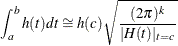
where ![$-\log [h(t)]$](images/statug_mcmc0554.png) assumes a minimum over
assumes a minimum over ![$[a, b]$](images/statug_mcmc0555.png) at an interior critical point c, and
at an interior critical point c, and  is the Hessian of ,
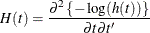
The minimum of the negative log integrand is found by using numerical optimization. By default, the CALL QUAD subroutine uses the quasi-Newton method. You can select other methods by using the quad_opt option.