The MCMC Procedure

Example 73.10 Missing at Random Analysis

This example illustrates how PROC MCMC treats missing at random (MAR) data. For a short overview of missing data problems, see the section Handling of Missing Data.

Researchers studied the effects of air pollution on respiratory disease in children. The response variable (y) represented whether a child exhibited wheezing symptoms; it was recorded as 1 for symptoms exhibited and 0 for no symptoms exhibited. City of residency (x1) and maternal smoking status (x2) were the explanatory variables. The variable x1 was coded as 1 if the child lived in the more polluted city, Steel City, and 0 if the child lived in Green Hills. The variable x2 was the number of cigarettes the mother reported that she smoked per day. Both the covariates contain missing values: 17 for x1 and 30 for x2, respectively. The total number of observations in the data set is 390. The following statements generate the data set air:


title 'Missing at Random Analysis';
data air;
   input y x1 x2 @@;
   datalines;
 0  0  0   0  0  0   0  1  0   0  0  0   0  0 11   0  1  7
 0  0  8   0  1 10   0  1  9   0  0  0   1  1  6   0  1 10
 0  1 12   0  0  .   0  0  0   0  1  0   0  1  7   1  1 15
 0  0  8   0  0  0   1  1  0   1  0  6   0  0  0   1  1 11
 0  0  0   1  0  0   1  0  5   0  0  8   0  0  0   0  1  9

   ... more lines ...   

 0  0 11   0  0  0   0  0  6   0  0 12   0  0 10   0  1 10
 0  1 11   0  0  9   1  0 11   0  1  7   0  0  7   0  0  0
 0  . 11   1  1  6   0  0  8   0  0  0   0  1 12   0  0  0
 0  1  0   1  1  8   0  0  0   0  1 11   0  1  0   0  1  8
 0  .  0   1  0  0   1  1 10   0  .  4   1  1 16   0  . 13
;

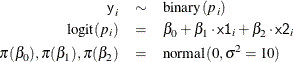
Suppose you want to fit a logistic regression model for whether the subject develops wheezing symptoms with density for the $i = 1, \ldots , 390$ subjects as follows:

$\begin{eqnarray*} {\Variable{y}}_ i & \sim & \mbox{binary}(p_ i) \\ \mbox{logit}(p_ i) & = & \beta _0 + \beta _1\cdot {\Variable{x1}}_ i + \beta _2\cdot {\Variable{x2}}_ i \\ \pi (\beta _0), \pi (\beta _1), \pi (\beta _2) & = & \mbox{normal}(0,\sigma ^2=10) \nonumber \end{eqnarray*}$

Suppose you specify a joint distribution of x1 and x2 in terms of the product of a conditional and marginal distribution; that is,

$\begin{eqnarray*} p({\Variable{x1}},{\Variable{x2}}|\balpha ) & = & p({\Variable{x1}}|{\Variable{x2}},\alpha _{10},\alpha _{11}) p({\Variable{x2}}|\alpha _{20}) \end{eqnarray*}$

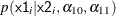where $p({\Variable{x1}}_ i | {\Variable{x2}}_ i, \alpha _{10},\alpha _{11})$ could be a logistic model and $p({\Variable{x2}}_ i | \alpha _{20})$ could be a Poisson distribution that models the following counts:

$\begin{eqnarray*} p({\Variable{x1}}_ i|{\Variable{x2}}_{i},\alpha _{10},\alpha _{11}) & = & \mbox{binary}(p_{c,i}) \\ \mbox{logit}(p_{c,i}) & = & \alpha _{10} + \alpha _{11}\cdot {\Variable{x2}}_{i} \\ \pi (\alpha _{10}), \pi (\alpha _{11}) & = & \mbox{normal}(0,\sigma ^2=10) \\ p({\Variable{x2}}_ i|\alpha _{20}) & = & \mbox{Poisson}(e^{\alpha _{20}}) \\ \pi (\alpha _{20}) & = & \mbox{normal}(0,\sigma ^2=2) \end{eqnarray*}$

The researchers are interested in interpreting how the odds of developing a wheeze changes for a child living in the more polluted city. The odds ratio can be written as the follows:

$\mbox{OR}_{{\Variable{x1}}} = \exp \left(\beta _1\right)$

Similarly, the odds ratio for the maternal smoking effect can be written as follows:

$\mbox{OR}_{{\Variable{x2}}} = \exp \left(\beta _2\right)$

The following statements fit a Bayesian logistic regression with missing covariates:

proc mcmc data=air seed=1181 nmc=10000 monitor=(_parms_ orx1 orx2)
   diag=none plots=none;
   parms beta0 -1 beta1 0.1 beta2 .01;
   parms alpha10 0 alpha11 0 alpha20 0;

   prior beta: alpha1: ~ normal(0,var=10);
   prior alpha20 ~ normal(0,var=2);

   beginnodata;
   pm = exp(alpha20);
   orx1 = exp(beta1);
   orx2 = exp(beta2);
   endnodata;
   model x2 ~ poisson(pm) monitor=(1 3 10);
   p1 = logistic(alpha10 + alpha11 * x2);
   model x1 ~ binary(p1) monitor=(random(3));
   p = logistic(beta0 + beta1*x1 + beta2*x2);
   model y ~ binary(p);
run;

The PARMS statements specify the parameters in the model and assign initial values to each of them. The PRIOR statements specify priors for all the model parameters. The notations beta: and alpha: in the PRIOR statements are shorthand for all variables that start with "beta," and "alpha," respectively. The shorthand notation is not necessary, but it keeps your code succinct.

The BEGINNODATA and ENDNODATA statements enclose three programming statements that calculate the Poisson mean (pm) and the two odds ratios (ORX1 and ORX2). These enclosed statements are independent of any data set variables, and they are run only once per iteration to reduce unnecessary observation-level computations.

The first MODEL statement assigns a Poisson likelihood with mean pm to x2. The statement models missing values in x2 automatically, creating one variable for each of the missing values, and augments them accordingly. By default, PROC MCMC does not output analyses of the posterior samples of the missing values. You can use the MONITOR= option to choose the missing values that you want to monitor. In the example, the first, third, and tenth missing values are monitored.

The P1 assignment statement calculates $p_{c.i}$ . The second MODEL statement assigns a binary likelihood with probability p1 and requests a random choice of three missing data variables of x1 to monitor.

The P assignment statement calculates $p_{i}$ in the logistic model. The third MODEL statement specifies the complete data likelihood function for Y.

Output 73.10.1 displays the number of observations read from the DATA= data set, the number of observations used in the analysis, and the "Missing Data Information" table. No observations were omitted from the data set in the analysis.

The "Missing Data Information" table lists the variables that contain missing values, which are x1 and x2, the number of missing observations in each variable, the observation indices of these missing values, and the sampling algorithms used. By default, the first 20 observation indices of each variable are printed in the table.

Output 73.10.1: Observation Information and Missing Data Information

Missing at Random Analysis

The MCMC Procedure

Number of Observations Read

Number of Observations Used

390

Missing Data Information Table
Variable	Number of Missing Obs	Observation Indices	Sampling Method
x2	30	14 41 50 55 59 66 71 83 88 90 118 158 174 175 178 183 196 203 210 212 ...	N-Metropolis
x1	17	50 92 93 167 194 231 273 296 303 304 308 330 349 373 385 388 390	Inverse CDF

There are 30 missing values in the variable x2, and 17 in x1. Internally, PROC MCMC creates 30 and 17 variables for the missing values in x2 and x1, respectively. The default naming convention for these missing values is to concatenate the response variable and the observation number. For example, the first missing value in x2 is the fourteenth observation, and the corresponding variable is x2_14.

Output 73.10.2 displays the summary and interval statistics for each parameter, the odds ratios, and the monitored missing values.

Output 73.10.2: Posterior Summary and Interval Statistics

Missing at Random Analysis

The MCMC Procedure

Posterior Summaries and Intervals
Parameter	N	Mean	Standard Deviation	95% HPD Interval
beta0	10000	-1.3732	0.2078	-1.7909	-0.9676
beta1	10000	0.4797	0.2387	0.0268	0.9491
beta2	10000	0.0156	0.0227	-0.0265	0.0642
alpha10	10000	-0.2166	0.1422	-0.4662	0.0874
alpha11	10000	0.0126	0.0201	-0.0267	0.0521
alpha20	10000	1.5635	0.0235	1.5199	1.6105
orx1	10000	1.6627	0.4094	0.9205	2.4493
orx2	10000	1.0160	0.0231	0.9739	1.0663
x2_14	10000	4.9022	2.2083	1.0000	9.0000
x2_50	10000	4.8924	2.1626	1.0000	9.0000
x2_90	10000	4.8263	2.0816	1.0000	8.0000
x1_296	10000	0.4160	0.4929	0	1.0000
x1_304	10000	0.4460	0.4971	0	1.0000
x1_373	10000	0.4443	0.4969	0	1.0000

The odds ratio for x1 is the multiplicative change in the odds of a child wheezing in Steel City compared to the odds of the child wheezing in Green Hills. The estimated odds ratio (ORX1) value is 1.6736 with a corresponding 95% equal-tail credible interval of $(1.0248, 2.5939)$ . City of residency is a significant factor in a child’s wheezing status. The estimated odds ratio for x2 is the multiplicative change in the odds of developing a wheeze for each additional reported cigarette smoked per day. The odds ratio of ORX2 indicates that the odds of a child developing a wheeze is 1.0150 times higher for each reported cigarette a mother smokes. The corresponding 95% equal-tail credible interval is $(0.9695,1.0619)$ . Since this interval contains the value 1, maternal smoking is not considered to be an influential effect.