The GLIMMIX Procedure
-
Overview

-
Getting Started
-
SyntaxPROC GLIMMIX StatementBY StatementCLASS StatementCODE StatementCONTRAST StatementCOVTEST StatementEFFECT StatementESTIMATE StatementFREQ StatementID StatementLSMEANS StatementLSMESTIMATE StatementMODEL StatementNLOPTIONS StatementOUTPUT StatementPARMS StatementRANDOM StatementSLICE StatementSTORE StatementWEIGHT StatementProgramming StatementsUser-Defined Link or Variance Function
-
DetailsGeneralized Linear Models TheoryGeneralized Linear Mixed Models TheoryGLM Mode or GLMM ModeStatistical Inference for Covariance ParametersDegrees of Freedom MethodsEmpirical Covariance ("Sandwich") EstimatorsExploring and Comparing Covariance MatricesProcessing by SubjectsRadial Smoothing Based on Mixed ModelsOdds and Odds Ratio EstimationParameterization of Generalized Linear Mixed ModelsResponse-Level Ordering and ReferencingComparing the GLIMMIX and MIXED ProceduresSingly or Doubly Iterative FittingDefault Estimation TechniquesDefault OutputNotes on Output StatisticsODS Table NamesODS Graphics
-
ExamplesBinomial Counts in Randomized BlocksMating Experiment with Crossed Random EffectsSmoothing Disease Rates; Standardized Mortality RatiosQuasi-likelihood Estimation for Proportions with Unknown DistributionJoint Modeling of Binary and Count DataRadial Smoothing of Repeated Measures DataIsotonic Contrasts for Ordered AlternativesAdjusted Covariance Matrices of Fixed EffectsTesting Equality of Covariance and Correlation MatricesMultiple Trends Correspond to Multiple Extrema in Profile LikelihoodsMaximum Likelihood in Proportional Odds Model with Random EffectsFitting a Marginal (GEE-Type) ModelResponse Surface Comparisons with Multiplicity AdjustmentsGeneralized Poisson Mixed Model for Overdispersed Count DataComparing Multiple B-SplinesDiallel Experiment with Multimember Random EffectsLinear Inference Based on Summary DataWeighted Multilevel Model for Survey DataQuadrature Method for Multilevel Model
- References
PROC GLIMMIX Statement
-
PROC GLIMMIX <options>;
The PROC GLIMMIX statement invokes the GLIMMIX procedure. Table 45.1 summarizes the options available in the PROC GLIMMIX statement. These and other options in the PROC GLIMMIX statement are then described fully in alphabetical order.
Table 45.1: PROC GLIMMIX Statement Options
|
Option |
Description |
|---|---|
|
Basic Options |
|
|
Specifies the input data set |
|
|
Determines estimation method |
|
|
Does not fit the model |
|
|
Includes scale parameter in optimization |
|
|
Determines computation of scale parameters in GLM models |
|
|
Determines the sort order of CLASS variables |
|
|
Writes |
|
|
Profile scale parameters from the optimization |
|
|
Displayed Output |
|
|
Displays the asymptotic correlation matrix of the covariance parameter estimates |
|
|
Displays the asymptotic covariance matrix of the covariance parameter estimates |
|
|
Displays the gradient of the objective function with respect to the parameter estimates |
|
|
Displays the Hessian matrix |
|
|
Adds estimates and gradients to the "Iteration History" |
|
|
Specifies the length of long effect names |
|
|
Shows data exclusions |
|
|
Suppresses "Class Level Information" completely or in part |
|
|
Requests odds ratios |
|
|
Produces ODS statistical graphics |
|
|
Writes subject-specific gradients to a SAS data set |
|
|
Optimization Options |
|
|
Specifies the number of optimizations |
|
|
Computational Options |
|
|
Constructs and solves mixed model equations using the Cholesky root of the |
|
|
Computes empirical ("sandwich") estimators |
|
|
Uses the expected Hessian matrix to compute the covariance matrix of nonprofiled parameters |
|
|
Affects the computation of information criteria |
|
|
Uses fixed-effects starting values via generalized linear model |
|
|
Sets the number of initial GLM steps |
|
|
Unbounds the covariance parameter estimates |
|
|
Does not use fixed-effects starting values via generalized linear model |
|
|
Applies Fisher scoring where applicable |
|
|
Bases the Hessian matrix in GLMMs on a modified scoring algorithm |
|
|
Singularity Tolerances |
|
|
Determines the absolute parameter estimate convergence criterion for PL |
|
|
Specifies significant digits in computing objective function |
|
|
Specifies the relative parameter estimate convergence criterion for PL |
|
|
Tunes singularity for Cholesky decompositions |
|
|
Tunes singularity for the residual variance |
|
|
Tunes general singularity criterion |
|
|
Debugging Output |
|
|
Lists model program and variables |
|
You can specify the following options in the PROC GLIMMIX statement.
- ABSPCONV=r
-
specifies an absolute parameter estimate convergence criterion for doubly iterative estimation methods. For such methods, the GLIMMIX procedure by default examines the relative change in parameter estimates between optimizations (see PCONV= ). The purpose of the ABSPCONV= criterion is to stop the process when the absolute change in parameter estimates is less than the tolerance criterion r. The criterion is based on fixed effects and covariance parameters.
Note that this convergence criterion does not affect the convergence criteria applied within any individual optimization. In order to change the convergence behavior within an optimization, you can change the ABSCONV=, ABSFCONV=, ABSGCONV=, ABSXCONV=, FCONV=, or GCONV= option in the NLOPTIONS statement.
- ASYCORR
-
produces the asymptotic correlation matrix of the covariance parameter estimates. It is computed from the corresponding asymptotic covariance matrix (see the description of the ASYCOV option, which follows).
- ASYCOV
-
requests that the asymptotic covariance matrix of the covariance parameter estimates be displayed. By default, this matrix is the observed inverse Fisher information matrix, which equals
 , where
  is the Hessian (second derivative) matrix of the objective function. The factor m equals 1 in a GLM and equals 2 in a GLMM.
When you use the SCORING= option and PROC GLIMMIX converges without stopping the scoring algorithm, the procedure uses the expected Hessian matrix to compute the covariance matrix instead of the observed Hessian. Regardless of whether a scoring algorithm is used or the number of scoring iterations has been exceeded, you can request that the asymptotic covariance matrix be based on the expected Hessian with the EXPHESSIAN option in the PROC GLIMMIX statement. If a residual scale parameter is profiled from the likelihood equation, the asymptotic covariance matrix is adjusted for the presence of this parameter; details of this adjustment process are found in Wolfinger, Tobias, and Sall (1994) and in the section Estimated Precision of Estimates.
-
CHOLESKY
CHOL -
requests that the mixed model equations be constructed and solved by using the Cholesky root of the
 matrix. This option applies only to estimation methods that involve mixed model equations. The Cholesky root algorithm has
greater numerical stability but also requires more computing resources. When the estimated matrix is not positive definite during a particular function evaluation, PROC GLIMMIX switches to the Cholesky algorithm
for that evaluation and returns to the regular algorithm if
matrix. This option applies only to estimation methods that involve mixed model equations. The Cholesky root algorithm has
greater numerical stability but also requires more computing resources. When the estimated matrix is not positive definite during a particular function evaluation, PROC GLIMMIX switches to the Cholesky algorithm
for that evaluation and returns to the regular algorithm if  becomes positive definite again. When the CHOLESKY option is in effect, the procedure applies the algorithm all the time.
- DATA=SAS-data-set
-
names the SAS data set to be used by PROC GLIMMIX. The default is the most recently created data set.
-
EMPIRICAL<=CLASSICAL | HC0>
EMPIRICAL<=DF | HC1>
EMPIRICAL<=MBN<(mbn-options)>>
EMPIRICAL<=ROOT | HC2>
EMPIRICAL<=FIRORES | HC3>
EMPIRICAL<=FIROEEQ<(r)>> -
requests that the covariance matrix of the parameter estimates be computed as one of the asymptotically consistent estimators, known as sandwich or empirical estimators. The name stems from the layering of the estimator. An empirically based estimate of the inverse variance of the parameter estimates (the "meat") is wrapped by the model-based variance estimate (the "bread").
Empirical estimators are useful for obtaining inferences that are not sensitive to the choice of the covariance model. In nonmixed models, they can help, for example, to allay the effects of variance heterogeneity on the tests of fixed effects. Empirical estimators can coarsely be grouped into likelihood-based and residual-based estimators. The distinction arises from the components used to construct the "meat" and "bread" of the estimator. If you specify the EMPIRICAL option without further qualifiers, the GLIMMIX procedure computes the classical sandwich estimator in the appropriate category.
Likelihood-Based Estimator
Let
 denote the second derivative matrix of the log likelihood for some parameter vector
  , and let
  denote the gradient of the log likelihood with respect to for the ith of m independent sampling units. The gradient for the entire data is
  . A sandwich estimator for the covariance matrix of
  can then be constructed as (White 1982)
![\[ \mb{H}(\widehat{\balpha })^{-1} \left( \sum _{i=1}^{m} \mb{g}_ i(\widehat{\balpha }) \mb{g}_ i(\widehat{\balpha })’ \right) \mb{H}(\widehat{\balpha })^{-1} \]](images/statug_glimmix0063.png)
If you fit a mixed model by maximum likelihood with Laplace or quadrature approximation (METHOD= LAPLACE , METHOD= QUAD ), the GLIMMIX procedure constructs this likelihood-based estimator when you choose EMPIRICAL=CLASSICAL. If you choose EMPIRICAL=MBN, the likelihood-based sandwich estimator is further adjusted (see the section Design-Adjusted MBN Estimator for details). Because Laplace and quadrature estimation in GLIMMIX includes the fixed-effects parameters and the covariance parameters in the optimization, this empirical estimator adjusts the covariance matrix of both types of parameters. The following empirical estimators are not available with METHOD= LAPLACE or with METHOD= QUAD : EMPIRICAL=DF, EMPIRICAL=ROOT, EMPIRICAL=FIRORES, and EMPIRICAL=FIROEEQ.
Residual-Based Estimators
For a general model, let
 denote the response with mean
  and variance
  , and let
  be the matrix of first derivatives of with respect to the fixed effects
  . The classical sandwich estimator (Huber 1967; White 1980) is
![\[ \widehat{\bOmega } \left( \sum _{i=1}^ m \widehat{\bD }_ i’ \widehat{\bSigma }_ i^{-1} \mb{e}_ i\mb{e}_ i’ \widehat{\bSigma }_ i^{-1} \widehat{\bD }_ i \right) \widehat{\bOmega } \]](images/statug_glimmix0067.png)
where
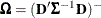 ,
,  , and m denotes the number of independent sampling units.
Since the expected value of
 does not equal
  , the classical sandwich estimator is biased, particularly if m is small. The estimator tends to underestimate the variance of
  . The EMPIRICAL=DF, ROOT, FIRORES, FIROEEQ, and MBN estimators are bias-corrected sandwich estimators. The DF estimator applies
a simple sample size adjustment. The ROOT, FIRORES, and FIROEEQ estimators are based on Taylor series approximations applied
to residuals and estimating equations. For uncorrelated data, the EMPIRICAL=FIRORES estimator can be motivated as a jackknife
estimator.
. The EMPIRICAL=DF, ROOT, FIRORES, FIROEEQ, and MBN estimators are bias-corrected sandwich estimators. The DF estimator applies
a simple sample size adjustment. The ROOT, FIRORES, and FIROEEQ estimators are based on Taylor series approximations applied
to residuals and estimating equations. For uncorrelated data, the EMPIRICAL=FIRORES estimator can be motivated as a jackknife
estimator.
In the case of a linear regression model, the various estimators reduce to the heteroscedasticity-consistent covariance matrix estimators (HCMM) of White (1980) and MacKinnon and White (1985). The classical estimator, HC0, was found to perform poorly in small samples. Based on simulations in regression models, MacKinnon and White (1985) and Long and Ervin (2000) strongly recommend the HC3 estimator. The sandwich estimators computed by the GLIMMIX procedure can be viewed as an extension of the HC0—HC3 estimators of MacKinnon and White (1985) to accommodate nonnormal data and correlated observations.
The MBN estimator, introduced as a residual-based estimator (Morel 1989; Morel, Bokossa, and Neerchal 2003), applies an additive adjustment to the residual crossproduct. It is controlled by three suboptions. The valid mbn-options are as follows: a sample size adjustment is applied when the DF suboption is in effect. The NODF suboption suppresses this component of the adjustment. The lower bound of the design effect parameter
 can be specified with the R= option. The magnitude of Morel’s
  parameter is partly determined with the D= option (
 ).
).
For details about the general expression for the residual-based estimators and their relationship, see the section Empirical Covariance ("Sandwich") Estimators. The MBN estimator and its parameters are explained for residual- and likelihood-based estimators in the section Design-Adjusted MBN Estimator.
The EMPIRICAL=DF estimator applies a simple, multiplicative correction factor to the classical estimator (Hinkley 1977). This correction factor is
![\[ c = \left\{ \begin{array}{ll} m / (m-k) & \quad m > k \\ 1 & \quad \mr{otherwise} \end{array} \right. \]](images/statug_glimmix0076.png)
where k is the rank of
 , and m equals the sum of all frequencies when PROC GLIMMIX is in
GLM mode and equals the number of subjects in
GLMM mode. For example, the following statements fit an overdispersed GLM:
, and m equals the sum of all frequencies when PROC GLIMMIX is in
GLM mode and equals the number of subjects in
GLMM mode. For example, the following statements fit an overdispersed GLM:
proc glimmix empirical;
   model y = x;
   random _residual_;
run;
PROC GLIMMIX is in GLM mode, and the individual observations are the independent sampling units from which the sandwich estimator is constructed. If you use a SUBJECT= effect in the RANDOM statement, however, the procedure fits the model in GLMM mode and the subjects represent the sampling units in the construction of the sandwich estimator. In other words, the following statements fit a GEE-type model with independence working covariance structure and subjects (clusters) defined by the levels of
ID:proc glimmix empirical; class id; model y = x; random _residual_ / subject=id type=vc; run;
See the section GLM Mode or GLMM Mode for information about how the GLIMMIX procedure determines the estimation mode.
The EMPIRICAL=ROOT estimator is based on the residual approximation in Kauermann and Carroll (2001), and the EMPIRICAL=FIRORES estimator is based on the approximation in Mancl and DeRouen (2001). The Kauermann and Carroll estimator requires the inverse square root of a nonsymmetric matrix. This square root matrix is obtained from the singular value decomposition in PROC GLIMMIX, and thus this sandwich estimator is computationally more demanding than others. In the linear regression case, the Mancl-DeRouen estimator can be motivated as a jackknife estimator, based on the "leave-one-out" estimates of
; see MacKinnon and White (1985) for details.
The EMPIRICAL=FIROEEQ estimator is based on approximating an unbiased estimating equation (Fay and Graubard 2001). It is computationally less demanding than the estimator of Kauermann and Carroll (2001) and, in certain balanced cases, gives identical results. The optional number
 is chosen to provide an upper bound on the correction factor. The default value for r is 0.75.
When you specify the EMPIRICAL option with a residual-based estimator, PROC GLIMMIX adjusts all standard errors and test statistics involving the fixed-effects parameters.
Sampling Units
Computation of an empirical variance estimator requires that the data can be processed by independent sampling units. This is always the case in GLMs. In this case, m, the number of independent units, equals the sum of the frequencies used in the analysis (see "Number of Observations" table). In GLMMs, empirical estimators can be computed only if the data comprise more than one subject as per the "Dimensions" table. See the section Processing by Subjects for information about how the GLIMMIX procedure determines whether the data can be processed by subjects. If a GLMM comprises only a single subject for a particular BY group, the model-based variance estimator is used instead of the empirical estimator, and a message is written to the log.
- EXPHESSIAN
-
requests that the expected Hessian matrix be used in computing the covariance matrix of the nonprofiled parameters. By default, the GLIMMIX procedure uses the observed Hessian matrix in computing the asymptotic covariance matrix of covariance parameters in mixed models and the covariance matrix of fixed effects in models without random effects. The EXPHESSIAN option is ignored if the (conditional) distribution is not a member of the exponential family or is unknown. It is also ignored in models for nominal data.
- FDIGITS=r
-
specifies the number of accurate digits in evaluations of the objective function. Fractional values are allowed. The default value is
 , where
  is the machine precision. The value of r is used to compute the interval size for the computation of finite-difference approximations of the derivatives of the objective
function. It is also used in computing the default value of the FCONV= option in the NLOPTIONS
statement.
is the machine precision. The value of r is used to compute the interval size for the computation of finite-difference approximations of the derivatives of the objective
function. It is also used in computing the default value of the FCONV= option in the NLOPTIONS
statement.
- GRADIENT
-
displays the gradient of the objective function with respect to the parameter estimates in the "Covariance Parameter Estimates" table and/or the "Parameter Estimates" table.
-
HESSIAN
HESS
H -
INFOCRIT=NONE | PQ | Q
IC=NONE | PQ | Q -
determines the computation of information criteria in the "Fit Statistics" table. The GLIMMIX procedure computes various information criteria that typically apply a penalty to the (possibly restricted) log likelihood, log pseudo-likelihood, or log quasi-likelihood that depends on the number of parameters and/or the sample size. If IC=NONE, these criteria are suppressed in the "Fit Statistics" table. This is the default for models based on pseudo-likelihoods.
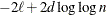
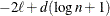
The AIC, AICC, BIC, CAIC, and HQIC fit statistics are various information criteria. AIC and AICC represent Akaike’s information criteria (Akaike 1974) and a small sample bias corrected version thereof (for AICC, see Hurvich and Tsai 1989; Burnham and Anderson 1998). BIC represents Schwarz’s Bayesian criterion (Schwarz 1978). Table 45.2 gives formulas for the criteria.
Table 45.2: Information Criteria
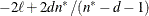
Here,
 denotes the maximum value of the (possibly restricted) log likelihood, log pseudo-likelihood, or log quasi-likelihood, d is the dimension of the model, and n,
  reflect the size of the data.
The IC=PQ option requests that the penalties include the number of fixed-effects parameters, when estimation in models with random effects is based on a residual (restricted) likelihood. For METHOD= MSPL, METHOD= MMPL, METHOD= LAPLACE , and METHOD= QUAD , IC=Q and IC=PQ produce the same results. IC=Q is the default for linear mixed models with normal errors, and the resulting information criteria are identical to the IC option in the MIXED procedure.
The quantities d, n, and
depend on the model and IC= option in the following way:
- GLM:
-
IC=Q and IC=PQ options have no effect on the computation.
-
d equals the number of parameters in the optimization whose solutions do not fall on the boundary or are otherwise constrained. The scale parameter is included, if it is part of the optimization. If you use the PARMS statement to place a hold on a scale parameter, that parameter does not count toward d.
-
n equals the sum of the frequencies (f) for maximum likelihood and quasi-likelihood estimation and
 for restricted maximum likelihood estimation.
-
equals n, unless
 , in which case
  .
.
-
- GLMM, IC=Q:
-
-
d equals the number of effective covariance parameters—that is, covariance parameters whose solution does not fall on the boundary. For estimation of an unrestricted objective function (METHOD= MMPL, METHOD= MSPL, METHOD= LAPLACE , METHOD= QUAD ), this value is incremented by
 .
.
-
n equals the effective number of subjects as displayed in the "Dimensions" table, unless this value equals 1, in which case n equals the number of levels of the first G-side RANDOM effect specified. If the number of effective subjects equals 1 and there are no G-side random effects, n is determined as
![\[ n = \left\{ \begin{array}{ll} f - \mr{rank}(\mb{X}) & \mr{METHOD=RMPL, METHOD=RSPL} \\ f & \mr{otherwise} \end{array} \right. \]](images/statug_glimmix0091.png)
where f is the sum of frequencies used.
-
equals f or
 (for METHOD=
RMPL and METHOD=
RSPL), unless this value is less than
(for METHOD=
RMPL and METHOD=
RSPL), unless this value is less than  , in which case .
-
- GLMM, IC=PQ:
-
For METHOD= MSPL, METHOD= MMPL, METHOD= LAPLACE , and METHOD= QUAD , the results are the same as for IC=Q. For METHOD= RSPL and METHOD= RMPL, d equals the number of effective covariance parameters plus
, and  equals . The formulas for the information criteria thus agree with Verbeke and Molenberghs (2000, Table 6.7, p. 74) and Vonesh and Chinchilli (1997, p. 263).
- INITGLM
-
requests that the estimates from a generalized linear model fit (a model without random effects) be used as the starting values for the generalized linear mixed model. This option is the default for METHOD= LAPLACE and METHOD= QUAD .
- INITITER=number
-
specifies the maximum number of iterations used when a generalized linear model is fit initially to derive starting values for the fixed effects; see the INITGLM option. By default, the initial fit involves at most four iteratively reweighted least squares updates. You can change the upper limit of initial iterations with number. If the model does not contain random effects, this option has no effect.
- ITDETAILS
-
adds parameter estimates and gradients to the "Iteration History" table.
- LIST
-
requests that the model program and variable lists be displayed. This is a debugging feature and is not normally needed. When you use programming statements to define your statistical model, this option enables you to examine the complete set of statements submitted for processing. See the section Programming Statements for more details about how to use SAS statements with the GLIMMIX procedure.
-
MAXLMMUPDATE=number
MAXOPT=number -
specifies the maximum number of optimizations for doubly iterative estimation methods based on linearizations. After each optimization, a new pseudo-model is constructed through a Taylor series expansion. This step is known as the linear mixed model update. The MAXLMMUPDATE option limits the number of updates and thereby limits the number of optimizations. If this option is not specified, number is set equal to the value specified in the MAXITER= option in the NLOPTIONS statement. If no MAXITER= value is given, number defaults to 20.
- METHOD=RSPL | MSPL | RMPL | MMPL | LAPLACE | QUAD<(quad-options)>
-
specifies the estimation method in a generalized linear mixed model (GLMM). The default is METHOD=RSPL.
Pseudo-Likelihood
Estimation methods ending in "PL" are pseudo-likelihood techniques. The first letter of the METHOD= identifier determines whether estimation is based on a residual likelihood ("R") or a maximum likelihood ("M"). The second letter identifies the expansion locus for the underlying approximation. Pseudo-likelihood methods for generalized linear mixed models can be cast in terms of Taylor series expansions (linearizations) of the GLMM. The expansion locus of the expansion is either the vector of random effects solutions ("S") or the mean of the random effects ("M"). The expansions are also referred to as the "S"ubject-specific and "M"arginal expansions. The abbreviation "PL" identifies the method as a pseudo-likelihood technique.
Residual methods account for the fixed effects in the construction of the objective function, which reduces the bias in covariance parameter estimates. Estimation methods involving Taylor series create pseudo-data for each optimization. Those data are transformed to have zero mean in a residual method. While the covariance parameter estimates in a residual method are the maximum likelihood estimates for the transformed problem, the fixed-effects estimates are (estimated) generalized least squares estimates. In a likelihood method that is not residual based, both the covariance parameters and the fixed-effects estimates are maximum likelihood estimates, but the former are known to have greater bias. In some problems, residual likelihood estimates of covariance parameters are unbiased.
For more information about linearization methods for generalized linear mixed models, see the section Pseudo-likelihood Estimation Based on Linearization.
Maximum Likelihood with Laplace Approximation
If you choose METHOD=LAPLACE with a generalized linear mixed model, PROC GLIMMIX approximates the marginal likelihood by using Laplace’s method. Twice the negative of the resulting log-likelihood approximation is the objective function that the procedure minimizes to determine parameter estimates. Laplace estimates typically exhibit better asymptotic behavior and less small-sample bias than pseudo-likelihood estimators. On the other hand, the class of models for which a Laplace approximation of the marginal log likelihood is available is much smaller compared to the class of models to which PL estimation can be applied.
To determine whether Laplace estimation can be applied in your model, consider the marginal distribution of the data in a mixed model
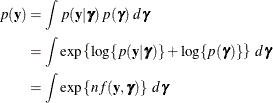
The function
 plays an important role in the Laplace approximation: it is a function of the joint distribution of the data and the random
effects (see the section Maximum Likelihood Estimation Based on Laplace Approximation). In order to construct a Laplace approximation, PROC GLIMMIX requires a conditional log-likelihood
plays an important role in the Laplace approximation: it is a function of the joint distribution of the data and the random
effects (see the section Maximum Likelihood Estimation Based on Laplace Approximation). In order to construct a Laplace approximation, PROC GLIMMIX requires a conditional log-likelihood  as well as the distribution of the G-side random effects. The random effects are always assumed to be normal with zero mean
and covariance structure determined by the RANDOM
statement. The conditional distribution is determined by the DIST=
option of the MODEL
statement or the default associated with a particular response type. Because a valid conditional distribution is required,
R-side random effects are not permitted for METHOD=LAPLACE in the GLIMMIX procedure. In other words, the GLIMMIX procedure
requires for METHOD=LAPLACE conditional independence without R-side overdispersion or covariance structure.
as well as the distribution of the G-side random effects. The random effects are always assumed to be normal with zero mean
and covariance structure determined by the RANDOM
statement. The conditional distribution is determined by the DIST=
option of the MODEL
statement or the default associated with a particular response type. Because a valid conditional distribution is required,
R-side random effects are not permitted for METHOD=LAPLACE in the GLIMMIX procedure. In other words, the GLIMMIX procedure
requires for METHOD=LAPLACE conditional independence without R-side overdispersion or covariance structure.
Because the marginal likelihood of the data is approximated numerically, certain features of the marginal distribution are not available—for example, you cannot display a marginal variance-covariance matrix. Also, the procedure includes both the fixed-effects parameters and the covariance parameters in the optimization for Laplace estimation. Consequently, this setting imposes some restrictions with respect to available options for Laplace estimation. Table 45.3 lists the options that are assumed for METHOD=LAPLACE, and Table 45.4 lists the options that are not compatible with this estimation method.
The section Maximum Likelihood Estimation Based on Laplace Approximation contains details about Laplace estimation in PROC GLIMMIX.
Maximum Likelihood with Adaptive Quadrature
If you choose METHOD=QUAD in a generalized linear mixed model, the GLIMMIX procedure approximates the marginal log likelihood with an adaptive Gauss-Hermite quadrature. Compared to METHOD=LAPLACE , the models for which parameters can be estimated by quadrature are further restricted. In addition to the conditional independence assumption and the absence of R-side covariance parameters, it is required that models suitable for METHOD=QUAD can be processed by subjects. (See the section Processing by Subjects about how the GLIMMIX procedure determines whether the data can be processed by subjects.) This in turn requires that all RANDOM statements have SUBJECT= effects and in the case of multiple SUBJECT= effects that these form a containment hierarchy.
In a containment hierarchy each effect is contained by another effect, and the effect contained by all is considered "the" effect for subject processing. For example, the SUBJECT= effects in the following statements form a containment hierarchy:
proc glimmix;
   class A B block;
   model y = A B A*B;
   random intercept / subject=block;
   random intercept / subject=A*block;
run;
The
blockeffect is contained in theA*blockinteraction and the data are processed byblock. The SUBJECT= effects in the following statements do not form a containment hierarchy:proc glimmix; class A B block; model y = A B A*B; random intercept / subject=block; random block / subject=A; run;
The section Maximum Likelihood Estimation Based on Adaptive Quadrature contains important details about the computations involved with quadrature approximations. The section Aspects Common to Adaptive Quadrature and Laplace Approximation contains information about issues that apply to Laplace and adaptive quadrature, such as the computation of the prediction variance matrix and the determination of starting values.
You can specify the following quad-options for METHOD=QUAD in parentheses:
- EBDETAILS
-
reports details about the empirical Bayes suboptimization process should this suboptimization fail.
- EBSSFRAC=r
-
specifies the step-shortening fraction to be used while computing empirical Bayes estimates of the random effects. The default value is r = 0.8, and it is required that
 .
.
- EBSSTOL=r
-
specifies the objective function tolerance for determining the cessation of step shortening while computing empirical Bayes estimates of the random effects,
 . The default value is r=1E–8.
- EBSTEPS=n
-
specifies the maximum number of Newton steps for computing empirical Bayes estimates of random effects,
 . The default value is n=50.
- EBSUBSTEPS=n
-
specifies the maximum number of step shortenings for computing empirical Bayes estimates of random effects. The default value is n=20, and it is required that
.
- EBTOL=r
-
specifies the convergence tolerance for empirical Bayes estimation,
. The default value is  , where is the machine precision. This default value equals approximately 1E–12 on most machines.
-
FASTQUAD
FQ -
requests the multilevel adaptive quadrature algorithm proposed by Pinheiro and Chao (2006). For a multilevel model, this algorithm reduces the number of random effects over which the integration for the marginal likelihood computation is carried out. The reduction in the dimension of the integral leads to the reduction in the number of conditional log-likelihood evaluations.
- INITPL=number
-
requests that adaptive quadrature commence after performing up to number pseudo-likelihood updates. The initial pseudo-likelihood (PL) steps (METHOD=MSPL) can be useful to provide good starting values for the quadrature algorithm. If you choose number large enough so that the initial PL estimation converges, the process is equivalent to starting a quadrature from the PL estimates of the fixed-effects and covariance parameters. Because this also makes available the PL random-effects solutions, the adaptive step of the quadrature that determines the number of quadrature points can take this information into account.
Note that you can combine the INITPL option with the NOINITGLM option in the PROC GLIMMIX statement to define a precise path for starting value construction to the GLIMMIX procedure. For example, the following statement generates starting values in these steps:
proc glimmix method=quad(initpl=5);
-
A GLM without random effects is fit initially to obtain as starting values for the fixed effects. The INITITER= option in the PROC GLIMMIX statement controls the number of iterations in this step.
-
Starting values for the covariance parameters are then obtained by MIVQUE0 estimation (Goodnight 1978a), using the fixed-effects parameter estimates from step 1.
-
With these values up to five pseudo-likelihood updates are computed.
-
The PL estimates for fixed-effects, covariance parameters, and the solutions for the random effects are then used to determine the number of quadrature points and used as the starting values for the quadrature.
The first step (GLM fixed-effects estimates) is omitted, if you modify the previous statement as follows:
proc glimmix method=quad(initpl=5) noinitglm;
The NOINITGLM option is the default of the pseudo-likelihood methods you select with the METHOD= option.
-
- QCHECK
-
performs an adaptive recalculation of the objective function (–2 log likelihood) at the solution. The increment of the quadrature points, starting from the number of points used in the optimization, follows the same rules as the determination of the quadrature point sequence at the starting values (see the QFAC= and QMAX= suboptions). For example, the following statement estimates the parameters based on a quadrature with seven nodes in each dimension:
proc glimmix method=quad(qpoints=7 qcheck);
Because the default search sequence is
 , the QCHECK option computes the –2 log likelihood at the converged solution for
  and 31 quadrature points and reports relative differences to the converged value and among successive values. The ODS table
produced by this option is named QuadCheck.
and 31 quadrature points and reports relative differences to the converged value and among successive values. The ODS table
produced by this option is named QuadCheck.
Caution: This option is useful to diagnose the sensitivity of the likelihood approximation at the solution. It does not diagnose the stability of the solution under changes in the number of quadrature points. For example, if increasing the number of points from 7 to 9 does not alter the objective function, this does not imply that a quadrature with 9 points would arrive at the same parameter estimates as a quadrature with 7 points.
- QFAC=r
-
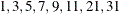
determines the step size for the quadrature point sequence. If the GLIMMIX procedure determines the quadrature nodes adaptively, the log likelihoods are computed for nodes in a predetermined sequence. If
 and
and  denote the values from the QMIN= and QMAX= suboptions, respectively, the sequence for values less than 11 is constructed
in increments of 2 starting at . Values greater than 11 are incremented in steps of r. The default value is r=10. The default sequence, without specifying the QMIN=, QMAX=, or QFAC= option, is thus . By contrast, the following statement evaluates the sequence
denote the values from the QMIN= and QMAX= suboptions, respectively, the sequence for values less than 11 is constructed
in increments of 2 starting at . Values greater than 11 are incremented in steps of r. The default value is r=10. The default sequence, without specifying the QMIN=, QMAX=, or QFAC= option, is thus . By contrast, the following statement evaluates the sequence  :
:
proc glimmix method=quad(qmin=8,qmax=51,qfac=20);
- QMAX=n
-
specifies an upper bound for the number of quadrature points. The default is n=31.
- QMIN=n
-
specifies a lower bound for the number of quadrature points. The default is n=1 and the value must be less than the QMAX= value.
- QPOINTS=n
-
determines the number of quadrature points in each dimension of the integral. Note that if there are r random effects for each subject, the GLIMMIX procedure evaluates
 conditional log likelihoods for each observation to compute one value of the objective function. Increasing the number of
quadrature nodes can substantially increase the computational burden. If you choose QPOINTS=1, the quadrature approximation
reduces to the Laplace approximation. If you do not specify the number of quadrature points, it is determined adaptively by
increasing the number of nodes at the starting values. See the section Aspects Common to Adaptive Quadrature and Laplace Approximation for details.
conditional log likelihoods for each observation to compute one value of the objective function. Increasing the number of
quadrature nodes can substantially increase the computational burden. If you choose QPOINTS=1, the quadrature approximation
reduces to the Laplace approximation. If you do not specify the number of quadrature points, it is determined adaptively by
increasing the number of nodes at the starting values. See the section Aspects Common to Adaptive Quadrature and Laplace Approximation for details.
- QTOL=r
-
specifies a relative tolerance criterion for the successive evaluation of log likelihoods for different numbers of quadrature points. When the GLIMMIX procedure determines the number of quadrature points adaptively, the number of nodes are increased until the QMAX=n limit is reached or until two successive evaluations of the log likelihood have a relative change of less than r. In the latter case, the lesser number of quadrature nodes is used for the optimization.
When you specify the FASTQUAD suboption to request the multilevel quadrature approximation for the marginal likelihood, gradients for the parameters in the optimization are computed by numerical finite-difference methods rather than analytically. These numerical gradients can in turn lead to Hessian matrices, log likelihoods, parameter estimates, and standard errors that are slightly different from what you would get without the FASTQUAD suboption.
The empirical estimators of covariance matrix of the parameter estimates that are produced by the EMPIRICAL option are not available when you specify the FASTQUAD suboption. Also, when you specify a nominal model, the FASTQUAD option is ignored.
The EBSSFRAC, EBSSTOL, EBSTEPS, EBSUBSTEPS, and EBTOL suboptions affect the suboptimization that leads to the empirical Bayes estimates of the random effects. Under normal circumstances, there is no reason to change from the default values. When the sub-optimizations fail, the optimization process can come to a halt. If the EBDETAILS option is in effect, you might be able to determine why the suboptimization fails and then adjust these values accordingly.
The QMIN, QMAX, QTOL, and QFAC suboptions determine the quadrature point search sequence for the adaptive component of estimation.
As for METHOD=LAPLACE , certain features of the marginal distribution are not available because the marginal likelihood of the data is approximated numerically. For example, you cannot display a marginal variance-covariance matrix. Also, the procedure includes both the fixed-effects and covariance parameters in the optimization for quadrature estimation. Consequently, this setting imposes some restrictions with respect to available options. Table 45.3 lists the options that are assumed for METHOD=QUAD and METHOD=LAPLACE , and Table 45.4 lists the options that are not compatible with these estimation methods.
Table 45.3: Defaults for METHOD=LAPLACE and METHOD=QUAD
Statement
Option
PROC GLIMMIX
NOPROFILE
PROC GLIMMIX
INITGLM
MODEL
NOCENTER
Table 45.4: Options Incompatible with METHOD=LAPLACE and METHOD=QUAD
Statement
Option
PROC GLIMMIX
EXPHESSIAN
PROC GLIMMIX
SCOREMOD
PROC GLIMMIX
SCORING
PROC GLIMMIX
PROFILE
MODEL
DDFM=KENWARDROGER
MODEL
DDFM=SATTERTHWAITE
MODEL
STDCOEF
RANDOM
RESIDUAL
RANDOM _RESIDUAL_
All R-side random effects
RANDOM
V
RANDOM
VC
RANDOM
VCI
RANDOM
VCORR
RANDOM
VI
In addition to the options displayed in Table 45.4, the NOBOUND option in the PROC GLIMMIX and the NOBOUND option in the PARMS statements are not available with METHOD=QUAD . Unbounding the covariance parameter estimates is possible with METHOD=LAPLACE , however.
No Random Effects Present
If the model does not contain G-side random effects or contains only a single overdispersion component, then the model belongs to the family of (overdispersed) generalized linear models if the distribution is known or the quasi-likelihood models for independent data if the distribution is not known. The GLIMMIX procedure then estimates model parameters by the following techniques:
-
normally distributed data: residual maximum likelihood
-
nonnormal data: maximum likelihood
-
data with unknown distribution: quasi-likelihood
The METHOD= specification then has only an effect with respect to the divisor used in estimating the overdispersion component. With a residual method, the divisor is f – k, where f denotes the sum of the frequencies and k is the rank of
 . Otherwise, the divisor is f.
- NAMELEN=number
-
specifies the length to which long effect names are shortened. The default and minimum value is 20.
- NOBOUND
-
requests the removal of boundary constraints on covariance and scale parameters in mixed models. For example, variance components have a default lower boundary constraint of 0, and the NOBOUND option allows their estimates to be negative.
The NOBOUND option cannot be used for adaptive quadrature estimation with METHOD= QUAD . The scaling of the quadrature abscissas requires an inverse Cholesky root that is possibly not well defined when the
matrix of the mixed model is negative definite or indefinite. The Laplace approximation (METHOD=
LAPLACE
) is not subject to this limitation.
- NOBSDETAIL
-
adds detailed information to the "Number of Observations" table to reflect how many observations were excluded from the analysis and for which reason.
- NOCLPRINT<=number>
-
suppresses the display of the "Class Level Information" table, if you do not specify number. If you specify number, only levels with totals that are less than number are listed in the table.
- NOFIT
-
suppresses fitting of the model. When the NOFIT option is in effect, PROC GLIMMIX produces the "Model Information," "Class Level Information," "Number of Observations," and "Dimensions" tables. These can be helpful to gauge the computational effort required to fit the model. For example, the "Dimensions" table informs you as to whether the GLIMMIX procedure processes the data by subjects, which is typically more computationally efficient than processing the data as a single subject. See the section Processing by Subjects for more information.
If you request a radial smooth with knot selection by k-d tree methods, PROC GLIMMIX also computes the knot locations of the smoother. You can then examine the knots without fitting the model. This enables you to try out different knot construction methods and bucket sizes. See the KNOTMETHOD =KDTREE option (and its suboptions) of the RANDOM statement.
If you combine the NOFIT option with the OUTDESIGN option, you can write the
and/or  matrix of your model to a SAS data set without fitting the model.
- NOINITGLM
-
requests that the starting values for the fixed effects not be obtained by first fitting a generalized linear model. This option is the default for the pseudo-likelihood estimation methods and for the linear mixed model. For the pseudo-likelihood methods, starting values can be implicitly defined based on an initial pseudo-data set derived from the data and the link function. For linear mixed models, starting values for the fixed effects are not necessary. The NOINITGLM option is useful in conjunction with the INITPL= suboption of METHOD= QUAD in order to perform initial pseudo-likelihood steps prior to an adaptive quadrature.
- NOITPRINT
- NOPROFILE
-
includes the scale parameter
 into the optimization for models that have such a parameter (see Table 45.20). By default, the GLIMMIX procedure profiles scale parameters from the optimization in mixed models. In generalized linear
models, scale parameters are not profiled.
into the optimization for models that have such a parameter (see Table 45.20). By default, the GLIMMIX procedure profiles scale parameters from the optimization in mixed models. In generalized linear
models, scale parameters are not profiled.
- NOREML
-
determines the denominator for the computation of the scale parameter in a GLM for normal data and for overdispersion parameters. By default, the GLIMMIX procedure computes the scale parameter for the normal distribution as
![\[ \widehat{\phi } = \sum _{i=1}^ n \frac{ f_ i (y_ i - \widehat{y}_ i)^2}{f - k} \]](images/statug_glimmix0108.png)
where k is the rank of
,  is the frequency associated with the ith observation, and
  . Similarly, the overdispersion parameter in an overdispersed GLM is estimated by the ratio of the Pearson statistic and
  . If the NOREML option is in effect, the denominators are replaced by f, the sum of the frequencies. In a GLM for normal data, this yields the maximum likelihood estimate of the error variance.
For this case, the NOREML option is a convenient way to change from REML to ML estimation.
. If the NOREML option is in effect, the denominators are replaced by f, the sum of the frequencies. In a GLM for normal data, this yields the maximum likelihood estimate of the error variance.
For this case, the NOREML option is a convenient way to change from REML to ML estimation.
In GLMM models fit by pseudo-likelihood methods, the NOREML option changes the estimation method to the nonresidual form. See the METHOD= option for the distinction between residual and nonresidual estimation methods.
-
ODDSRATIO
OR -
requests that odds ratios be added to the output when applicable. Odds ratios and their confidence limits are reported only for models with logit, cumulative logit, or generalized logit link. Specifying the ODDSRATIO option in the PROC GLIMMIX statement has the same effect as specifying the ODDSRATIO option in the MODEL statement and in all LSMEANS statements. Note that the ODDSRATIO option in the MODEL statement has several suboptions that enable you to construct customized odds ratios. These suboptions are available only through the MODEL statement. For details about the interpretation and computation of odds and odds ratios with the GLIMMIX procedure, see the section Odds and Odds Ratio Estimation.
- ORDER=DATA | FORMATTED | FREQ | INTERNAL
-
specifies the sort order for the levels of the classification variables (which are specified in the CLASS statement).
This ordering determines which parameters in the model correspond to each level in the data, so the ORDER= option can be useful when you use CONTRAST or ESTIMATE statements. This option applies to the levels for all classification variables, except when you use the (default) ORDER=FORMATTED option with numeric classification variables that have no explicit format. In that case, the levels of such variables are ordered by their internal value.
The ORDER= option can take the following values:
Value of ORDER=
Levels Sorted By
DATA
Order of appearance in the input data set
FORMATTED
External formatted value, except for numeric variables with no explicit format, which are sorted by their unformatted (internal) value
FREQ
Descending frequency count; levels with the most observations come first in the order
INTERNAL
Unformatted value
By default, ORDER=FORMATTED. For ORDER=FORMATTED and ORDER=INTERNAL, the sort order is machine-dependent.
When the response variable appears in a CLASS statement, the ORDER= option in the PROC GLIMMIX statement applies to its sort order. Specification of a response-option in the MODEL statement overrides the ORDER= option in the PROC GLIMMIX statement. For example, in the following statements the sort order of the
wheezevariable is determined by the formatted value (default):proc glimmix order=data; class city; model wheeze = city age / dist=binary s; run;
The ORDER= option in the PROC GLIMMIX statement has no effect on the sort order of the
wheezevariable because it does not appear in the CLASS statement. However, in the following statements the sort order of thewheezevariable is determined by the order of appearance in the input data set because the response variable appears in the CLASS statement:proc glimmix order=data; class city wheeze; model wheeze = city age / dist=binary s; run;
For more information about sort order, see the chapter on the SORT procedure in the Base SAS Procedures Guide and the discussion of BY-group processing in SAS Language Reference: Concepts.
- OUTDESIGN<(options)> <=SAS-data-set>
-
creates a data set that contains the contents of the
and  matrix. If the data are processed by subjects as shown in the "Dimensions" table, then the matrix saved to the data set corresponds to a single subject. By default, the GLIMMIX procedure includes in the OUTDESIGN
data set the and matrix (if present) and the variables in the input data set. You can specify the following options in parentheses to control the contents of the OUTDESIGN data set:
matrix. If the data are processed by subjects as shown in the "Dimensions" table, then the matrix saved to the data set corresponds to a single subject. By default, the GLIMMIX procedure includes in the OUTDESIGN
data set the and matrix (if present) and the variables in the input data set. You can specify the following options in parentheses to control the contents of the OUTDESIGN data set:
- NAMES
-
produces tables associating columns in the OUTDESIGN data set with fixed-effects parameter estimates and random-effects solutions.
- NOMISS
-
excludes from the OUTDESIGN data set observations that were not used in the analysis.
- NOVAR
-
excludes from the OUTDESIGN data set variables from the input data set. Variables listed in the BY and ID statements and variables needed for identification of SUBJECT= effects are always included in the OUTDESIGN data set.
- X<=prefix>
-
saves the contents of the
matrix. The optional prefix is used to name the columns. The default naming prefix is "_X".
- Z<=prefix>
-
saves the contents of the
matrix. The optional prefix is used to name the columns. The default naming prefix is "_Z".
The order of the observations in the OUTDESIGN data set is the same as the order of the input data set. If you do not specify a data set with the OUTDESIGN option, the procedure uses the
DATAnconvention to name the data set. - PCONV=r
-
specifies the parameter estimate convergence criterion for doubly iterative estimation methods. The GLIMMIX procedure applies this criterion to fixed-effects estimates and covariance parameter estimates. Suppose
 denotes the estimate of the ith parameter at the uth optimization. The procedure terminates the doubly iterative process if the largest value
![\[ 2 \times \frac{ | \widehat{\psi }_ i^{(u)} - \widehat{\psi }_ i^{(u-1)} |}{ |\widehat{\psi }_ i^{(u)}| + |\widehat{\psi }_ i^{(u-1)}|} \]](images/statug_glimmix0113.png)
is less than r. To check an absolute convergence criteria as well, you can set the ABSPCONV= option in the PROC GLIMMIX statement. The default value for r is 1E8 times the machine epsilon, a product that equals about 1E–8 on most machines.
Note that this convergence criterion does not affect the convergence criteria applied within any individual optimization. In order to change the convergence behavior within an optimization, you can use the ABSCONV=, ABSFCONV=, ABSGCONV=, ABSXCONV=, FCONV=, or GCONV= option in the NLOPTIONS statement.
-
PLOTS <(global-plot-options)> <=plot-request <(options)>>
PLOTS <(global-plot-options)> <=(plot-request <(options)> <... plot-request <(options)>>)> -
requests that the GLIMMIX procedure produce statistical graphics via ODS Graphics.
ODS Graphics must be enabled before plots can be requested. For example:
ods graphics on;

proc glimmix data=plants;
   class Block Type;
   model StemLength = Block Type;
   lsmeans type / diff=control plots=controlplot;
run;

ods graphics off;
For more information about enabling and disabling ODS Graphics, see the section Enabling and Disabling ODS Graphics in Chapter 21: Statistical Graphics Using ODS.
For examples of the basic statistical graphics produced by the GLIMMIX procedure and aspects of their computation and interpretation, see the section ODS Graphics in this chapter. You can also request statistical graphics for least squares means through the PLOTS option in the LSMEANS statement, which gives you more control over the display compared to the PLOTS option in the PROC GLIMMIX statement.
Global Plot Options
The global-plot-options apply to all relevant plots generated by the GLIMMIX procedure. The global-plot-options supported by the GLIMMIX procedure are as follows:
Specific Plot Options
The following listing describes the specific plots and their options.
- ALL
-
requests that all plots appropriate for the analysis be produced. In models with G-side random effects, residual plots are based on conditional residuals (by using the BLUPs of random effects) on the linear (linked) scale. Plots of least squares means differences are produced for LSMEANS statements without options that would contradict such a display.
-
ANOMPLOT
ANOM -
requests an analysis of means display in which least squares means are compared against an average least squares mean (Ott 1967; Nelson 1982, 1991, 1993). See the DIFF= option in the LSMEANS statement for the computation of this average. Least squares mean ANOM plots are produced only for those fixed effects that are listed in LSMEANS statements that have options that do not contradict the display. For example, if you request ANOM plots with the PLOTS= option in the PROC GLIMMIX statement, the following LSMEANS statements produce analysis of mean plots for effects
AandC:lsmeans A / diff=anom; lsmeans B / diff; lsmeans C;
The DIFF option in the second LSMEANS statement implies all pairwise differences.
When differences against the average LS-mean are adjusted for multiplicity with the ADJUST= NELSON option in the LSMEANS statement, the ANOMPLOT display is adjusted accordingly.
- BOXPLOT <(boxplot-options)>
-
requests box plots for the effects in your model that consist of classification effects only. Note that these effects can involve more than one classification variable (interaction and nested effects), but cannot contain any continuous variables. By default, the BOXPLOT request produces box plots of (conditional) residuals for the qualifying effects in the MODEL and RANDOM statements. See the discussion of the boxplot-options in a later section for information about how to tune your box plot request.
-
CONTROLPLOT
CONTROL -
requests a display in which least squares means are visually compared against a reference level. LS-mean control plots are produced only for those fixed effects that are listed in LSMEANS statements that have options that do not contradict with the display. For example, the following statements produce control plots for effects
AandCif you specify PLOTS=CONTROL in the PROC GLIMMIX statement:lsmeans A / diff=control('1'); lsmeans B / diff; lsmeans C;The DIFF option in the second LSMEANS statement implies all pairwise differences.
When differences against a control level are adjusted for multiplicity with the ADJUST= option in the LSMEANS statement, the control plot display is adjusted accordingly.
-
DIFFPLOT<(diffplot-options)>
DIFFOGRAM <(diffplot-options)>
DIFF<(diffplot-options)> -
requests a display of all pairwise least squares mean differences and their significance. When constructed from arithmetic means, the display is also known as a "mean-mean scatter plot" (Hsu 1996; Hsu and Peruggia 1994). For each comparison a line segment, centered at the LS-means in the pair, is drawn. The length of the segment corresponds to the projected width of a confidence interval for the least squares mean difference. Segments that fail to cross the 45-degree reference line correspond to significant least squares mean differences.
If you specify the ADJUST= option in the LSMEANS statement, the lengths of the line segments are adjusted for multiplicity.
LS-mean difference plots are produced only for those fixed effects listed in LSMEANS statements that have options that do not conflict with the display. For example, the following statements request differences against a control level for the
Aeffect, all pairwise differences for theBeffect, and the least squares means for theCeffect:lsmeans A / diff=control('1'); lsmeans B / diff; lsmeans C;The DIFF= type in the first statement contradicts a display of all pairwise differences. Difference plots are produced only for the B and C effects if you specify PLOTS=DIFF in the PROC GLIMMIX statement.
You can specify the following diffplot-options. The ABS and NOABS options determine the positioning of the line segments in the plot. When the ABS option is in effect (this is the default) all line segments are shown on the same side of the reference line. The NOABS option separates comparisons according to the sign of the difference. The CENTER option marks the center point for each comparison. This point corresponds to the intersection of two least squares means. The NOLINES option suppresses the display of the line segments that represent the confidence bounds for the differences of the least squares means. The NOLINES option implies the CENTER option. The default is to draw line segments in the upper portion of the plot area without marking the center point.
- MEANPLOT<(meanplot-options)>
-
requests a display of the least squares means of effects specified in LSMEANS statements. The following meanplot-options affect the display. Upper and lower confidence limits are plotted when the CL option is used. When the CLBAND option is in effect, confidence limits are shown as bands and the means are connected. By default, least squares means are not joined by lines. You can achieve that effect with the JOIN or CONNECT option. Least squares means are displayed in the same order in which they appear in the "Least Squares Means" table. You can change that order for plotting purposes with the ASCENDING and DESCENDING options. The ILINK option requests that results be displayed on the inverse linked (the data) scale.
Note that there is also a MEANPLOT suboption of the PLOTS= option in the LSMEANS statement. In addition to the meanplot-options just described, you can also specify classification effects that give you more control over the display of interaction means through the PLOTBY= and SLICEBY= options. To display interaction means, you typically want to use the MEANPLOT option in the LSMEANS statement. For example, the next statement requests a plot in which the levels of
Aare placed on the horizontal axis and the means that belong to the same level ofBare joined by lines:lsmeans A*B / plot=meanplot(sliceby=b join);
- NONE
-
requests that no plots be produced.
- ODDSRATIO <(oddsratioplot-options)>
-
requests a display of odds ratios and their confidence limits when the link function permits the computation of odds ratios (see the ODDSRATIO option in the MODEL statement). Possible suboptions of the ODDSRATIO plot request are described below under the heading "Odds Ratio Plot Options."
- RESIDUALPANEL<(residualplot-options)>
-
requests a paneled display constructed from raw residuals. The panel consists of a plot of the residuals against the linear predictor or predicted mean, a histogram with normal density overlaid, a Q-Q plot, and a box plot of the residuals. The residualplot-options enable you to specify which type of residual is being graphed. These are further discussed below under the heading "Residual Plot Options."
- STUDENTPANEL<(residualplot-options)>
-
requests a paneled display constructed from studentized residuals. The same panel organization is applied as for the RESIDUALPANEL plot type.
- PEARSONPANEL<(residualplot-options)>
-
requests a paneled display constructed from Pearson residuals. The same panel organization is applied as for the RESIDUALPANEL plot type.
Residual Plot Options
The residualplot-options apply to the RESIDUALPANEL, STUDENTPANEL, and PEARSONPANEL displays. The primary function of these options is to control which type of a residual to display. The four types correspond to keyword-options as for output statistics in the OUTPUT statement. The residualplot-options take on the following values:
You can list a plot request one or more times with different options. For example, the following statements request a panel of marginal raw residuals, individual plots generated from a panel of the conditional raw residuals, and a panel of marginal studentized residuals:
ods graphics on;
proc glimmix plots=(ResidualPanel(marginal)
                    ResidualPanel(unpack conditional)
                    StudentPanel(marginal));
The default is to compute conditional residuals on the linear scale if the model contains G-side random effects (BLUP NOILINK). Not all combinations of the BLUP/NOBLUP and ILINK/NOILINK suboptions are possible for all residual types and models. For details, see the description of output statistics for the OUTPUT statement. Pearson residuals are always displayed against the linear predictor; all other residuals are graphed versus the linear predictor if the NOILINK suboption is in effect (default), and against the corresponding prediction on the mean scale if the ILINK option is in effect. See Table 45.15 for a definition of the residual quantities and exclusions.
Box Plot Options
The boxplot-options determine whether box plots are produced for residuals or for residuals and observed values, and for which model effects the box plots are constructed. The available boxplot-options are as follows:
By default, box plots of residuals are constructed from the raw conditional residuals (on the linked scale) in linear mixed models and from Pearson residuals in all other models. Note that not all combinations of the BLUP/NOBLUP and ILINK/NOILINK suboptions are possible for all residual types and models. For details, see the description of output statistics for the OUTPUT statement.
Odds Ratio Plot Options
The oddsratioplot-options determine the display of odds ratios and their confidence limits. The computation of the odds ratios follows the ODDSRATIO option in the MODEL statement. The available oddsratioplot-options are as follows:
- LOGBASE= 2 | E | 10
-
log-scales the odds ratio axis.
- NPANELPOS=n
-
provides the capability to break an odds ratio plot into multiple graphics having at most
 odds ratios per graphic. If n is positive, then the number of odds ratios per graphic is balanced. If n is negative, then no balancing of the number of odds ratios takes place. For example, suppose you want to display 21 odds
ratios. Then NPANELPOS=20 displays two plots, the first with 11 and the second with 10 odds ratios, and NPANELPOS=–20 displays
20 odds ratios in the first plot and a single odds ratio in the second. If n=0 (this is the default), then all odds ratios are displayed in a single plot.
odds ratios per graphic. If n is positive, then the number of odds ratios per graphic is balanced. If n is negative, then no balancing of the number of odds ratios takes place. For example, suppose you want to display 21 odds
ratios. Then NPANELPOS=20 displays two plots, the first with 11 and the second with 10 odds ratios, and NPANELPOS=–20 displays
20 odds ratios in the first plot and a single odds ratio in the second. If n=0 (this is the default), then all odds ratios are displayed in a single plot.
- ORDER=ASCENDING | DESCENDING
-
displays the odds ratios in sorted order. By default the odds ratios are displayed in the order in which they appear in the "Odds Ratio Estimates" table.
- RANGE=(<min> <,max>) | CLIP
-
specifies the range of odds ratios to display. If you specify RANGE=CLIP, then the confidence intervals are clipped and the range contains the minimum and maximum odds ratios. By default the range of view captures the extent of the odds ratio confidence intervals.
- STATS
-
adds the numeric values of the odds ratio and its confidence limits to the graphic.


- PROFILE
-
requests that scale parameters be profiled from the optimization, if possible. This is the default for generalized linear mixed models. In generalized linear models with normally distributed data, you can use the PROFILE option to request profiling of the residual variance.
- SCOREMOD
-
requests that the Hessian matrix in GLMMs be based on a modified scoring algorithm, provided that PROC GLIMMIX is in scoring mode when the Hessian is evaluated. The procedure is in scoring mode during iteration, if the optimization technique requires second derivatives, the SCORING=n option is specified, and the iteration count has not exceeded n. The procedure also computes the expected (scoring) Hessian matrix when you use the EXPHESSIAN option in the PROC GLIMMIX statement.
The SCOREMOD option has no effect if the SCORING= or EXPHESSIAN option is not specified. The nature of the SCOREMOD modification to the expected Hessian computation is shown in Table 45.23, in the section Pseudo-likelihood Estimation Based on Linearization. The modification can improve the convergence behavior of the GLMM compared to standard Fisher scoring and can provide a better approximation of the variability of the covariance parameters. For more details, see the section Estimated Precision of Estimates.
- SCORING=number
-
requests that Fisher scoring be used in association with the estimation method up to iteration number. By default, no scoring is applied. When you use the SCORING= option and PROC GLIMMIX converges without stopping the scoring algorithm, the procedure uses the expected Hessian matrix to compute approximate standard errors for the covariance parameters instead of the observed Hessian. If necessary, the standard errors of the covariance parameters as well as the output from the ASYCOV and ASYCORR options are adjusted.
If scoring stopped prior to convergence and you want to use the expected Hessian matrix in the computation of standard errors, use the EXPHESSIAN option in the PROC GLIMMIX statement.
Scoring is not possible in models for nominal data. It is also not possible for GLMs with unknown distribution or for those outside the exponential family. If you perform quasi-likelihood estimation, the GLIMMIX procedure is always in scoring mode and the SCORING= option has no effect. See the section Quasi-likelihood for Independent Data for a description of the types of models where GLIMMIX applies quasi-likelihood estimation.
The SCORING= option has no effect for optimization methods that do not involve second derivatives. See the TECHNIQUE= option in the NLOPTIONS statement and the section Choosing an Optimization Algorithm in Chapter 19: Shared Concepts and Topics, for details about first- and second-order algorithms.
- SINGCHOL=number
-
tunes the singularity criterion in Cholesky decompositions. The default is 1E4 times the machine epsilon; this product is approximately 1E–12 on most computers.
- SINGRES=number
-
sets the tolerance for which the residual variance is considered to be zero. The default is 1E4 times the machine epsilon; this product is approximately 1E–12 on most computers.
- SINGULAR=number
-
tunes the general singularity criterion applied by the GLIMMIX procedure in divisions and inversions. The default is 1E4 times the machine epsilon; this product is approximately 1E–12 on most computers.
- STARTGLM
-
is an alias of the INITGLM option.
-
SUBGRADIENT<=SAS-data-set>
SUBGRAD<=SAS-data-set> -
creates a data set with information about the gradient of the objective function. The contents and organization of the SUBGRADIENT= data set depend on the type of model. The following paragraphs describe the SUBGRADIENT= data set for the two major estimation modes. See the section GLM Mode or GLMM Mode for details about the estimation modes of the GLIMMIX procedure.
- GLMM Mode
-
If the GLIMMIX procedure operates in GLMM mode, the SUBGRADIENT= data set contains as many observations as there are usable subjects in the analysis. The maximum number of usable subjects is displayed in the "Dimensions" table. Gradient information is not written to the data set for subjects who do not contribute valid observations to the analysis. Note that the objective function in the "Iteration History" table is in terms of the –2 log (residual, pseudo-) likelihood. The gradients in the SUBGRADIENT= data set are gradients of that objective function.
The gradients are evaluated at the final solution of the estimation problem. If the GLIMMIX procedure fails to converge, then the information in the SUBGRADIENT= data set corresponds to the gradient evaluated at the last iteration or optimization.
The number of gradients saved to the SUBGRADIENT= data set equals the number of parameters in the optimization. For example, with METHOD= LAPLACE or METHOD= QUAD the fixed-effects parameters and the covariance parameters take part in the optimization. The order in which the gradients appear in the data set equals the order in which the gradients are displayed when the ITDETAILS option is in effect: gradients for fixed-effects parameters precede those for covariance parameters, and gradients are not reported for singular columns in the
 matrix. In models where the residual variance is profiled from the optimization, a subject-specific gradient is not reported
for the residual variance. To decompose this gradient by subjects, add the NOPROFILE
option in the PROC GLIMMIX
statement. When the subject-specific gradients in the SUBGRADIENT= data set are summed, the totals equal the values reported
by the GRADIENT
option.
matrix. In models where the residual variance is profiled from the optimization, a subject-specific gradient is not reported
for the residual variance. To decompose this gradient by subjects, add the NOPROFILE
option in the PROC GLIMMIX
statement. When the subject-specific gradients in the SUBGRADIENT= data set are summed, the totals equal the values reported
by the GRADIENT
option.
- GLM Mode
-
When you fit a generalized linear model (GLM) or a GLM with overdispersion, the SUBGRADIENT= data set contains the observation-wise gradients of the negative log-likelihood function with respect to the parameter estimates. Note that this corresponds to the objective function in GLMs as displayed in the "Iteration History" table. However, the gradients displayed in the "Iteration History" for GLMs—when the ITDETAILS option is in effect—are possibly those of the centered and scaled coefficients. The gradients reported in the "Parameter Estimates" table and in the SUBGRADIENT= data set are gradients with respect to the uncentered and unscaled coefficients.
The gradients are evaluated at the final estimates. If the model does not converge, the gradients contain missing values. The gradients appear in the SUBGRADIENT= data set in the same order as in the "Parameter Estimates" table, with singular columns removed.
The variables from the input data set are added to the SUBGRADIENT= data set in GLM mode. The data set is organized in the same way as the input data set; observations that do not contribute to the analysis are transferred to the SUBGRADIENT= data set, but gradients are calculated only for observations that take part in the analysis. If you use an ID statement, then only the variables in the ID statement are transferred to the SUBGRADIENT= data set.