The GLIMMIX Procedure
-
Overview

-
Getting Started
-
SyntaxPROC GLIMMIX StatementBY StatementCLASS StatementCODE StatementCONTRAST StatementCOVTEST StatementEFFECT StatementESTIMATE StatementFREQ StatementID StatementLSMEANS StatementLSMESTIMATE StatementMODEL StatementNLOPTIONS StatementOUTPUT StatementPARMS StatementRANDOM StatementSLICE StatementSTORE StatementWEIGHT StatementProgramming StatementsUser-Defined Link or Variance Function
-
DetailsGeneralized Linear Models TheoryGeneralized Linear Mixed Models TheoryGLM Mode or GLMM ModeStatistical Inference for Covariance ParametersDegrees of Freedom MethodsEmpirical Covariance ("Sandwich") EstimatorsExploring and Comparing Covariance MatricesProcessing by SubjectsRadial Smoothing Based on Mixed ModelsOdds and Odds Ratio EstimationParameterization of Generalized Linear Mixed ModelsResponse-Level Ordering and ReferencingComparing the GLIMMIX and MIXED ProceduresSingly or Doubly Iterative FittingDefault Estimation TechniquesDefault OutputNotes on Output StatisticsODS Table NamesODS Graphics
-
ExamplesBinomial Counts in Randomized BlocksMating Experiment with Crossed Random EffectsSmoothing Disease Rates; Standardized Mortality RatiosQuasi-likelihood Estimation for Proportions with Unknown DistributionJoint Modeling of Binary and Count DataRadial Smoothing of Repeated Measures DataIsotonic Contrasts for Ordered AlternativesAdjusted Covariance Matrices of Fixed EffectsTesting Equality of Covariance and Correlation MatricesMultiple Trends Correspond to Multiple Extrema in Profile LikelihoodsMaximum Likelihood in Proportional Odds Model with Random EffectsFitting a Marginal (GEE-Type) ModelResponse Surface Comparisons with Multiplicity AdjustmentsGeneralized Poisson Mixed Model for Overdispersed Count DataComparing Multiple B-SplinesDiallel Experiment with Multimember Random EffectsLinear Inference Based on Summary DataWeighted Multilevel Model for Survey DataQuadrature Method for Multilevel Model
- References
Example 45.4 Quasi-likelihood Estimation for Proportions with Unknown Distribution
Wedderburn (1974) analyzes data on the incidence of leaf blotch (Rhynchosporium secalis) on barley.
The data represent the percentage of leaf area affected in a two-way layout with 10 barley varieties at nine sites. The following DATA step converts these data to proportions, as analyzed in McCullagh and Nelder (1989, Ch. 9.2.4). The purpose of the analysis is to make comparisons among the varieties, adjusted for site effects.
data blotch;
   array p{9} pct1-pct9;
   input variety pct1-pct9;
   do site = 1 to 9;
      prop = p{site}/100;
      output;
   end;
   drop pct1-pct9;
   datalines;
1  0.05  0.00  1.25  2.50  5.50  1.00  5.00  5.00 17.50
2  0.00  0.05  1.25  0.50  1.00  5.00  0.10 10.00 25.00
3  0.00  0.05  2.50  0.01  6.00  5.00  5.00  5.00 42.50
4  0.10  0.30 16.60  3.00  1.10  5.00  5.00  5.00 50.00
5  0.25  0.75  2.50  2.50  2.50  5.00 50.00 25.00 37.50
6  0.05  0.30  2.50  0.01  8.00  5.00 10.00 75.00 95.00
7  0.50  3.00  0.00 25.00 16.50 10.00 50.00 50.00 62.50
8  1.30  7.50 20.00 55.00 29.50  5.00 25.00 75.00 95.00
9  1.50  1.00 37.50  5.00 20.00 50.00 50.00 75.00 95.00
10 1.50 12.70 26.25 40.00 43.50 75.00 75.00 75.00 95.00
;
Little is known about the distribution of the leaf area proportions. The outcomes are not binomial proportions, because they
do not represent the ratio of a count over a total number of Bernoulli trials. However, because the mean proportion  for variety j on site i must lie in the interval
 ![$[0,1]$](images/statug_glimmix0955.png) , you can commence the analysis with a model that treats
, you can commence the analysis with a model that treats Prop as a "pseudo-binomial" variable:
![\begin{align*} \mr{E}[\Variable{Prop}_{ij}] & = \mu _{ij} \\ \mu _{ij} & = 1/(1+\exp \{ -\eta _{ij}\} ) \\ \eta _{ij} & = \beta _0 + \alpha _ i + \tau _ j \\ \mr{Var}[\Variable{Prop}_{ij}] & = \phi \mu _{ij}(1-\mu _{ij}) \end{align*}](images/statug_glimmix1011.png)
Here,  is the linear predictor for variety j on site i,
  denotes the ith site effect, and
  denotes the jth barley variety effect. The logit of the expected leaf area proportions is linearly related to these effects. The variance
function of the model is that of a binomial(n,) variable, and
denotes the jth barley variety effect. The logit of the expected leaf area proportions is linearly related to these effects. The variance
function of the model is that of a binomial(n,) variable, and  is an overdispersion parameter. The moniker "pseudo-binomial" derives not from the pseudo-likelihood methods used to estimate
the parameters in the model, but from treating the response variable as if it had first and second moment properties akin
to a binomial random variable.
is an overdispersion parameter. The moniker "pseudo-binomial" derives not from the pseudo-likelihood methods used to estimate
the parameters in the model, but from treating the response variable as if it had first and second moment properties akin
to a binomial random variable.
The model is fit in the GLIMMIX procedure with the following statements:
proc glimmix data=blotch;
   class site variety;
   model prop = site variety / link=logit dist=binomial;
   random _residual_;
   lsmeans variety / diff=control('1');
run;
The MODEL
statement specifies the distribution as binomial and the logit link. Because the variance function of the binomial distribution
is 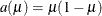 , you use the statement
random _residual_;
to specify the
scale parameter . The LSMEANS
statement requests estimates of the least squares means for the barley variety. The DIFF
=CONTROL(’1’) option requests tests of least squares means differences against the first variety.
The "Model Information" table in Output 45.4.1 describes the model and methods used in fitting the statistical model. It is assumed here that the data are binomial proportions.
Output 45.4.1: Model Information in Pseudo-binomial Analysis
The "Class Level Information" table in Output 45.4.2 lists the number of levels of the Site and Variety effects and their values. All 90 observations read from the data are used in the analysis.
Output 45.4.2: Class Levels and Number of Observations
In Output 45.4.3, the "Dimensions" table shows that the model does not contain G-side random effects. There is a single covariance parameter,
which corresponds to . The "Optimization Information" table shows that the optimization comprises 18 parameters (Output 45.4.3). These correspond to the 18 nonsingular columns of the  matrix.
Output 45.4.3: Model Fit in Pseudo-binomial Analysis
There are significant site and variety effects in this model based on the approximate Type III F tests (Output 45.4.4).
Output 45.4.4: Tests of Site and Variety Effects in Pseudo-binomial Analysis
Output 45.4.5 displays the Variety least squares means for this analysis. These are obtained by averaging
![\[ \mr{logit}(\widehat{\mu }_{ij}) = \widehat{\eta }_{ij} \]](images/statug_glimmix1015.png)
across the sites. In other words, LS-means are computed on the linked scale where the model effects are additive. Note that the least squares means are ordered by variety. The estimate of the expected proportion of infected leaf area for the first variety is
![\[ \widehat{\mu }_{.,1} = \frac{1}{1+\exp \{ 4.38\} } = 0.0124 \]](images/statug_glimmix1016.png)
and that for the last variety is
![\[ \widehat{\mu }_{.,10} = \frac{1}{1+\exp \{ 0.127\} } = 0.468 \]](images/statug_glimmix1017.png)
Output 45.4.5: Variety Least Squares Means in Pseudo-binomial Analysis
| variety Least Squares Means | |||||
|---|---|---|---|---|---|
| variety | Estimate | Standard Error |
DF | t Value | Pr > |t| |
| 1 | -4.3800 | 0.5643 | 72 | -7.76 | <.0001 |
| 2 | -4.2300 | 0.5383 | 72 | -7.86 | <.0001 |
| 3 | -3.6906 | 0.4623 | 72 | -7.98 | <.0001 |
| 4 | -3.3319 | 0.4239 | 72 | -7.86 | <.0001 |
| 5 | -2.7653 | 0.3768 | 72 | -7.34 | <.0001 |
| 6 | -2.0089 | 0.3320 | 72 | -6.05 | <.0001 |
| 7 | -1.8095 | 0.3228 | 72 | -5.61 | <.0001 |
| 8 | -1.0380 | 0.2960 | 72 | -3.51 | 0.0008 |
| 9 | -0.8800 | 0.2921 | 72 | -3.01 | 0.0036 |
| 10 | -0.1270 | 0.2808 | 72 | -0.45 | 0.6523 |
Because of the ordering of the least squares means, the differences against the first variety are also ordered from smallest to largest (Output 45.4.6).
Output 45.4.6: Variety Differences against the First Variety
| Differences of variety Least Squares Means | ||||||
|---|---|---|---|---|---|---|
| variety | _variety | Estimate | Standard Error | DF | t Value | Pr > |t| |
| 2 | 1 | 0.1501 | 0.7237 | 72 | 0.21 | 0.8363 |
| 3 | 1 | 0.6895 | 0.6724 | 72 | 1.03 | 0.3086 |
| 4 | 1 | 1.0482 | 0.6494 | 72 | 1.61 | 0.1109 |
| 5 | 1 | 1.6147 | 0.6257 | 72 | 2.58 | 0.0119 |
| 6 | 1 | 2.3712 | 0.6090 | 72 | 3.89 | 0.0002 |
| 7 | 1 | 2.5705 | 0.6065 | 72 | 4.24 | <.0001 |
| 8 | 1 | 3.3420 | 0.6015 | 72 | 5.56 | <.0001 |
| 9 | 1 | 3.5000 | 0.6013 | 72 | 5.82 | <.0001 |
| 10 | 1 | 4.2530 | 0.6042 | 72 | 7.04 | <.0001 |
This analysis depends on your choice for the variance function that was implied by the binomial distribution. You can diagnose the distributional assumption by examining various graphical diagnostics measures. The following statements request a panel display of the Pearson-type residuals:
ods graphics on;
ods select PearsonPanel;
proc glimmix data=blotch plots=pearsonpanel;
   class site variety;
   model prop = site variety / link=logit dist=binomial;
   random _residual_;
run;
ods graphics off;
Output 45.4.7 clearly indicates that the chosen variance function is not appropriate for these data. As  approaches zero or one, the variability in the residuals is less than that implied by the binomial variance function.
Output 45.4.7: Panel of Pearson-Type Residuals in Pseudo-binomial Analysis
To remedy this situation, McCullagh and Nelder (1989) consider instead the variance function
![\[ \mr{Var}[\Variable{Prop}_{ij}] = \mu _{ij}^2 (1-\mu _{ij})^2 \]](images/statug_glimmix1018.png)
Imagine two varieties with  and
and  . Under the binomial variance function, the variance of the proportion for variety k is 2.77 times larger than that for variety i. Under the revised model this ratio increases to
  .
.
The analysis of the revised model is obtained with the next set of GLIMMIX statements. Because you need to model a variance function that does not correspond to any of the built-in distributions, you need to supply a function with an assignment to the automatic variable _VARIANCE_. The GLIMMIX procedure then considers the distribution of the data as unknown. The corresponding estimation technique is quasi-likelihood. Because this model does not include an extra scale parameter, you can drop the RANDOM _RESIDUAL_ statement from the analysis.
ods graphics on;
ods select ModelInfo FitStatistics LSMeans Diffs PearsonPanel;
proc glimmix data=blotch plots=pearsonpanel;
   class site variety;
   _variance_ = _mu_**2 * (1-_mu_)**2;
   model prop = site variety / link=logit;
   lsmeans variety / diff=control('1');
run;
ods graphics off;
The "Model Information" table in Output 45.4.8 now displays the distribution as "Unknown," because of the assignment made in the GLIMMIX statements to _VARIANCE_. The table also shows the expression evaluated as the variance function.
Output 45.4.8: Model Information in Quasi-likelihood Analysis
The fit statistics of the model are now expressed in terms of the log quasi-likelihood. It is computed as
![\[ \sum _{i=1}^{9}\, \sum _{j=1}^{10} \int _{y_{ij}}^{\mu _{ij}} \frac{y_{ij} - t}{t^2(1-t)^2} \, dt \]](images/statug_glimmix1022.png)
Twice the negative of this sum equals –85.74, which is displayed in the "Fit Statistics" table (Output 45.4.9).
The scaled Pearson statistic is now 0.99. Inclusion of an extra scale parameter would have little or no effect on the results.
Output 45.4.9: Fit Statistics in Quasi-likelihood Analysis
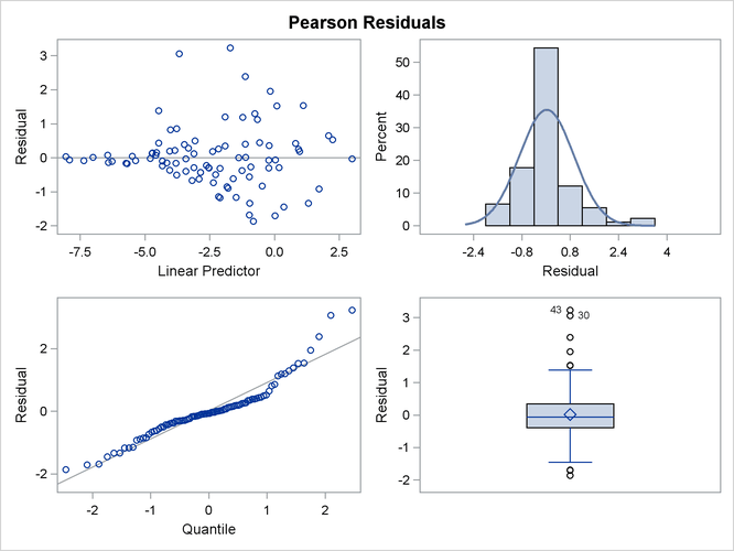
The panel of Pearson-type residuals now shows a much more adequate distribution for the residuals and a reduction in the number of outlying residuals (Output 45.4.10).
Output 45.4.10: Panel of Pearson-Type Residuals (Quasi-likelihood)
The least squares means are no longer ordered in size by variety (Output 45.4.11). For example,  . Under the revised model, the second variety has a greater percentage of its leaf area covered by blotch, compared to the
first variety. Varieties 5 and 6 and varieties 8 and 9 show similar reversal in ranking.
. Under the revised model, the second variety has a greater percentage of its leaf area covered by blotch, compared to the
first variety. Varieties 5 and 6 and varieties 8 and 9 show similar reversal in ranking.
Output 45.4.11: Variety Least Squares Means in Quasi-likelihood Analysis
| variety Least Squares Means | |||||
|---|---|---|---|---|---|
| variety | Estimate | Standard Error |
DF | t Value | Pr > |t| |
| 1 | -4.0453 | 0.3333 | 72 | -12.14 | <.0001 |
| 2 | -4.5126 | 0.3333 | 72 | -13.54 | <.0001 |
| 3 | -3.9664 | 0.3333 | 72 | -11.90 | <.0001 |
| 4 | -3.0912 | 0.3333 | 72 | -9.27 | <.0001 |
| 5 | -2.6927 | 0.3333 | 72 | -8.08 | <.0001 |
| 6 | -2.7167 | 0.3333 | 72 | -8.15 | <.0001 |
| 7 | -1.7052 | 0.3333 | 72 | -5.12 | <.0001 |
| 8 | -0.7827 | 0.3333 | 72 | -2.35 | 0.0216 |
| 9 | -0.9098 | 0.3333 | 72 | -2.73 | 0.0080 |
| 10 | -0.1580 | 0.3333 | 72 | -0.47 | 0.6369 |
Interestingly, the standard errors are constant among the LS-means (Output 45.4.11) and among the LS-means differences (Output 45.4.12). This is due to the fact that for the logit link
![\[ \frac{\partial \mu }{\partial \eta } = \mu (1-\mu ) \]](images/statug_glimmix1024.png)
which cancels with the square root of the variance function in the estimating equations. The analysis is thus orthogonal.
Output 45.4.12: Variety Differences in Quasi-likelihood Analysis
| Differences of variety Least Squares Means | ||||||
|---|---|---|---|---|---|---|
| variety | _variety | Estimate | Standard Error | DF | t Value | Pr > |t| |
| 2 | 1 | -0.4673 | 0.4714 | 72 | -0.99 | 0.3249 |
| 3 | 1 | 0.07885 | 0.4714 | 72 | 0.17 | 0.8676 |
| 4 | 1 | 0.9541 | 0.4714 | 72 | 2.02 | 0.0467 |
| 5 | 1 | 1.3526 | 0.4714 | 72 | 2.87 | 0.0054 |
| 6 | 1 | 1.3286 | 0.4714 | 72 | 2.82 | 0.0062 |
| 7 | 1 | 2.3401 | 0.4714 | 72 | 4.96 | <.0001 |
| 8 | 1 | 3.2626 | 0.4714 | 72 | 6.92 | <.0001 |
| 9 | 1 | 3.1355 | 0.4714 | 72 | 6.65 | <.0001 |
| 10 | 1 | 3.8873 | 0.4714 | 72 | 8.25 | <.0001 |