The GLIMMIX Procedure
-
Overview

-
Getting Started
-
SyntaxPROC GLIMMIX StatementBY StatementCLASS StatementCODE StatementCONTRAST StatementCOVTEST StatementEFFECT StatementESTIMATE StatementFREQ StatementID StatementLSMEANS StatementLSMESTIMATE StatementMODEL StatementNLOPTIONS StatementOUTPUT StatementPARMS StatementRANDOM StatementSLICE StatementSTORE StatementWEIGHT StatementProgramming StatementsUser-Defined Link or Variance Function
-
DetailsGeneralized Linear Models TheoryGeneralized Linear Mixed Models TheoryGLM Mode or GLMM ModeStatistical Inference for Covariance ParametersDegrees of Freedom MethodsEmpirical Covariance ("Sandwich") EstimatorsExploring and Comparing Covariance MatricesProcessing by SubjectsRadial Smoothing Based on Mixed ModelsOdds and Odds Ratio EstimationParameterization of Generalized Linear Mixed ModelsResponse-Level Ordering and ReferencingComparing the GLIMMIX and MIXED ProceduresSingly or Doubly Iterative FittingDefault Estimation TechniquesDefault OutputNotes on Output StatisticsODS Table NamesODS Graphics
-
ExamplesBinomial Counts in Randomized BlocksMating Experiment with Crossed Random EffectsSmoothing Disease Rates; Standardized Mortality RatiosQuasi-likelihood Estimation for Proportions with Unknown DistributionJoint Modeling of Binary and Count DataRadial Smoothing of Repeated Measures DataIsotonic Contrasts for Ordered AlternativesAdjusted Covariance Matrices of Fixed EffectsTesting Equality of Covariance and Correlation MatricesMultiple Trends Correspond to Multiple Extrema in Profile LikelihoodsMaximum Likelihood in Proportional Odds Model with Random EffectsFitting a Marginal (GEE-Type) ModelResponse Surface Comparisons with Multiplicity AdjustmentsGeneralized Poisson Mixed Model for Overdispersed Count DataComparing Multiple B-SplinesDiallel Experiment with Multimember Random EffectsLinear Inference Based on Summary DataWeighted Multilevel Model for Survey DataQuadrature Method for Multilevel Model
- References
Example 45.11 Maximum Likelihood in Proportional Odds Model with Random Effects
The data for this example are taken from Gilmour, Anderson, and Rae (1987) and concern the foot shape of 2,513 lambs that represent 34 sires. The foot shape of the animals was scored in three ordered
categories. The following DATA step lists the data in multivariate form, where each observation corresponds to a sire and
contains the outcomes for the three response categories in the variables k1, k2, and k3. For example, for the first sire the first foot shape category was observed for 52 of its offspring, foot shape category
2 was observed for 25 lambs, and none of its offspring was rated in foot shape category 3. The variables yr, b1, b2, and b3 represent contrasts of fixed effects.
data foot_mv;
   input yr b1 b2 b3 k1 k2 k3;
   sire = _n_;
   datalines;
  1  1  0  0  52 25  0
  1  1  0  0  49 17  1
  1  1  0  0  50 13  1
  1  1  0  0  42  9  0
  1  1  0  0  74 15  0
  1  1  0  0  54  8  0
  1  1  0  0  96 12  0
  1 -1  1  0  57 52  9
  1 -1  1  0  55 27  5
  1 -1  1  0  70 36  4
  1 -1  1  0  70 37  3
  1 -1  1  0  82 21  1
  1 -1  1  0  75 19  0
  1 -1 -1  0  17 12 10
  1 -1 -1  0  13 23  3
  1 -1 -1  0  21 17  3
 -1  0  0  1  37 41 23
 -1  0  0  1  47 24 12
 -1  0  0  1  46 25  9
 -1  0  0  1  79 32 11
 -1  0  0  1  50 23  5
 -1  0  0  1  63 18  8
 -1  0  0 -1  30 20  9
 -1  0  0 -1  31 33  3
 -1  0  0 -1  28 18  4
 -1  0  0 -1  42 27  4
 -1  0  0 -1  35 22  2
 -1  0  0 -1  33 18  3
 -1  0  0 -1  35 17  4
 -1  0  0 -1  26 13  2
 -1  0  0 -1  37 15  2
 -1  0  0 -1  36 14  1
 -1  0  0 -1  63 20  3
 -1  0  0 -1  41  8  1
;
In order to analyze these data as multinomial data with PROC GLIMMIX, the data need to be arranged in univariate form. The
following DATA step creates three observations from each record in data set foot_mv and stores the category counts in the variable count:
data footshape; set foot_mv;
   array k{3};
   do Shape = 1 to 3;
      count = k{Shape};
      output;
   end;
   drop k:;
run;
Because the sires were selected at random, a model for the three-category response with fixed regression effects for yr, b1–b3, and with random sire effects is considered. Because the response categories are ordered, a proportional odds model is chosen
(McCullagh 1980). Gilmour, Anderson, and Rae (1987) consider various analyses for these data. The following GLIMMIX statements fit a model with probit link for the cumulative
probabilities by maximum likelihood where the marginal log likelihood is approximated by adaptive quadrature:
proc glimmix data=footshape method=quad;
   class sire;
   model Shape = yr b1 b2 b3 / s link=cumprobit dist=multinomial;
   random int / sub=sire s cl;
   ods output Solutionr=solr;
   freq count;
run;
The number of observations that share a particular response and covariate pattern (variable count) is used in the FREQ
statement. The S
and CL
options request solutions for the sire effects. These are output to the data set solr for plotting.
The "Model Information" table shows that the parameters are estimated by maximum likelihood and that the marginal likelihood is approximated by Gauss-Hermite quadrature (Output 45.11.1).
Output 45.11.1: Model and Data Information
| Model Information | |
|---|---|
| Data Set | WORK.FOOTSHAPE |
| Response Variable | Shape |
| Response Distribution | Multinomial (ordered) |
| Link Function | Cumulative Probit |
| Variance Function | Default |
| Frequency Variable | count |
| Variance Matrix Blocked By | sire |
| Estimation Technique | Maximum Likelihood |
| Likelihood Approximation | Gauss-Hermite Quadrature |
| Degrees of Freedom Method | Containment |
The distribution of the data is multinomial with ordered categories. The ordering is implied by the choice of a link function for the cumulative probabilities. Because a frequency variable is specified, the number of observations as well as the number of frequencies is displayed. Observations with zero frequency—that is, foot shape categories that were not observed for a particular sire are not used in the analysis. The "Response Profile Table" shows the ordering of the response variable and gives a breakdown of the frequencies by category.
Output 45.11.2: Information about the Size of the Optimization Problem
With METHOD= QUAD , the "Dimensions" and "Optimization Information" tables are particularly important, because for this estimation methods both fixed effects and covariance parameters participate in the optimization (Output 45.11.2). For GLM models the optimization involves the fixed effects and possibly a single scale parameter. For mixed models the fixed effects are typically profiled from the optimization. Laplace and quadrature estimations are exceptions to these rules. Consequently, there are seven parameters in this optimization, corresponding to six fixed effects and one variance component. The variance component has a lower bound of 0. Also, because the fixed effects are part of the optimizations, PROC GLIMMIX initially performs a few GLM iterations to obtain starting values for the fixed effects. You can control the number of initial iterations with the INITITER= option in the PROC GLIMMIX statement.
The last entry in the "Optimization Information" table shows that—at the starting values—PROC GLIMMIX determined that a single quadrature point is sufficient to approximate the marginal log likelihood with the required accuracy. This approximation is thus identical to the Laplace method that is available with METHOD= LAPLACE .
For METHOD= LAPLACE and METHOD= QUAD , the GLIMMIX procedure produces fit statistics based on the conditional and marginal distribution (Output 45.11.3). Within the limits of the numeric likelihood approximation, the information criteria shown in the "Fit Statistics" table can be used to compare models, and the –2 log likelihood can be used to compare among nested models (nested with respect to fixed effects and/or the covariance parameters).
Output 45.11.3: Marginal and Conditional Fit Statistics
The variance of the sire effect is estimated as 0.04849 with estimated asymptotic standard error of 0.01673 (Output 45.11.4). Based on the magnitude of the estimate relative to the standard error, one might conclude that there is significant sire-to-sire
variability. Because parameter estimation is based on maximum likelihood, a formal test of the hypothesis of no sire variability
is possible. The category cutoffs for the cumulative probabilities are 0.3781 and 1.6435. Except for b3, all fixed effects contrasts are significant.
Output 45.11.4: Parameter Estimates
| Solutions for Fixed Effects | ||||||
|---|---|---|---|---|---|---|
| Effect | Shape | Estimate | Standard Error |
DF | t Value | Pr > |t| |
| Intercept | 1 | 0.3781 | 0.04907 | 29 | 7.71 | <.0001 |
| Intercept | 2 | 1.6435 | 0.05930 | 29 | 27.72 | <.0001 |
| yr | 0.1422 | 0.04834 | 2478 | 2.94 | 0.0033 | |
| b1 | 0.3781 | 0.07154 | 2478 | 5.28 | <.0001 | |
| b2 | 0.3157 | 0.09709 | 2478 | 3.25 | 0.0012 | |
| b3 | -0.09887 | 0.06508 | 2478 | -1.52 | 0.1289 | |
A likelihood ratio test for the sire variability can be carried out by adding a COVTEST statement to the PROC GLIMMIX statements (Output 45.11.5):
ods select FitStatistics CovParms Covtests;
proc glimmix data=footshape method=quad;
   class sire;
   model Shape = yr b1 b2 b3 / link=cumprobit dist=multinomial;
   random int / sub=sire;
   covtest GLM;
   freq count;
run;
The statement
covtest GLM;
compares the fitted model to a generalized linear model for independent data by removing the sire variance component from the model. Equivalently, you can specify
covtest 0;
which compares the fitted model against one where the sire variance is fixed at zero.
Output 45.11.5: Likelihood Ratio Test for Sire Variance
The –2 Log Likelihood in the reduced model without the sire effect is 3915.29. Compared to the corresponding marginal fit statistic in the full model (3870.12), this results in a chi-square statistic of 45.17. Because the variance component for the sire effect has a natural lower bound of zero, PROC GLIMMIX performs the likelihood ratio test as a one-sided test. As indicated by the note, the p-value for this test is computed from a mixture of chi-square distributions, applying the results of Self and Liang (1987). There is significant evidence that the model without sire random effects does not fit the data as well.
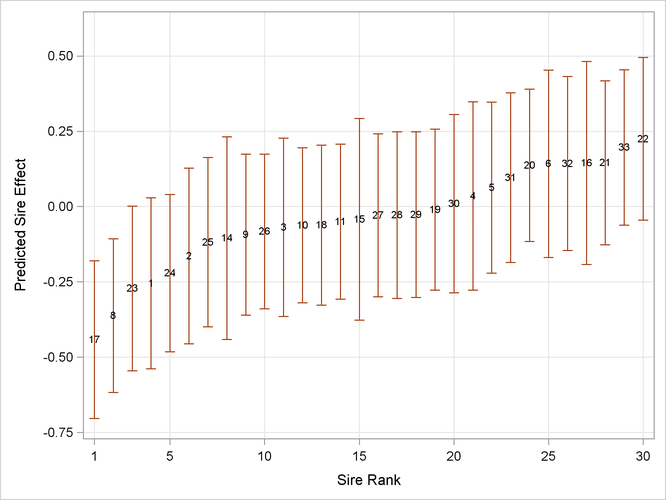
In studies of heritability, one is often interested to rank individuals according to some measure of "breeding value." The following statements display the empirical Bayes estimates of the sire effects from ML estimation by quadrature along with prediction standard error bars (Output 45.11.6):
proc sort data=solr;
   by Estimate;
run;
data solr; set solr;
   length sire $2;
   obs  = _n_;
   sire = left(substr(Subject,6,2));
run;
proc sgplot data=solr;
   scatter x=obs y=estimate /
         markerchar  = sire
         yerrorupper = upper
         yerrorlower = lower;
   xaxis grid label='Sire Rank' values=(1 5 10 15 20 25 30);
   yaxis grid label='Predicted Sire Effect';
run;
Output 45.11.6: Ranked Predicted Sire Effects and Prediction Standard Errors