The GLIMMIX Procedure
-
Overview

-
Getting Started
-
SyntaxPROC GLIMMIX StatementBY StatementCLASS StatementCODE StatementCONTRAST StatementCOVTEST StatementEFFECT StatementESTIMATE StatementFREQ StatementID StatementLSMEANS StatementLSMESTIMATE StatementMODEL StatementNLOPTIONS StatementOUTPUT StatementPARMS StatementRANDOM StatementSLICE StatementSTORE StatementWEIGHT StatementProgramming StatementsUser-Defined Link or Variance Function
-
DetailsGeneralized Linear Models TheoryGeneralized Linear Mixed Models TheoryGLM Mode or GLMM ModeStatistical Inference for Covariance ParametersDegrees of Freedom MethodsEmpirical Covariance ("Sandwich") EstimatorsExploring and Comparing Covariance MatricesProcessing by SubjectsRadial Smoothing Based on Mixed ModelsOdds and Odds Ratio EstimationParameterization of Generalized Linear Mixed ModelsResponse-Level Ordering and ReferencingComparing the GLIMMIX and MIXED ProceduresSingly or Doubly Iterative FittingDefault Estimation TechniquesDefault OutputNotes on Output StatisticsODS Table NamesODS Graphics
-
ExamplesBinomial Counts in Randomized BlocksMating Experiment with Crossed Random EffectsSmoothing Disease Rates; Standardized Mortality RatiosQuasi-likelihood Estimation for Proportions with Unknown DistributionJoint Modeling of Binary and Count DataRadial Smoothing of Repeated Measures DataIsotonic Contrasts for Ordered AlternativesAdjusted Covariance Matrices of Fixed EffectsTesting Equality of Covariance and Correlation MatricesMultiple Trends Correspond to Multiple Extrema in Profile LikelihoodsMaximum Likelihood in Proportional Odds Model with Random EffectsFitting a Marginal (GEE-Type) ModelResponse Surface Comparisons with Multiplicity AdjustmentsGeneralized Poisson Mixed Model for Overdispersed Count DataComparing Multiple B-SplinesDiallel Experiment with Multimember Random EffectsLinear Inference Based on Summary DataWeighted Multilevel Model for Survey DataQuadrature Method for Multilevel Model
- References
RANDOM Statement
-
RANDOM random-effects </ options>;
Using notation from Notation for the Generalized Linear Mixed Model, the RANDOM statement defines the  matrix of the mixed model, the random effects in the
  vector, the structure of
  , and the structure of
  .
.
The matrix is constructed exactly like the  matrix for the fixed effects, and the matrix is constructed to correspond to the effects constituting . The structures of and are defined by using the TYPE=
option described on . The random effects can be classification or continuous effects, and multiple RANDOM statements are
possible.
matrix for the fixed effects, and the matrix is constructed to correspond to the effects constituting . The structures of and are defined by using the TYPE=
option described on . The random effects can be classification or continuous effects, and multiple RANDOM statements are
possible.
Some reserved keywords have special significance in the random-effects list.
You can specify INTERCEPT (or INT) as a random effect to indicate the intercept. PROC GLIMMIX does not include the intercept
in the RANDOM statement by default as it does in the MODEL
statement.
You can specify the _RESIDUAL_ keyword (or RESID, RESIDUAL, _RESID_) before the option slash (/) to indicate a residual-type
(R-side) random component that defines the  matrix. Basically, the _RESIDUAL_ keyword takes the place of the random-effect if you want to specify
R-side variances and covariance structures. These keywords take precedence over variables in the data set with the same name. If your data or the covariance structure requires that
an effect is specified, you can use the RESIDUAL
option to instruct the GLIMMIX procedure to model the R-side variances and covariances.
matrix. Basically, the _RESIDUAL_ keyword takes the place of the random-effect if you want to specify
R-side variances and covariance structures. These keywords take precedence over variables in the data set with the same name. If your data or the covariance structure requires that
an effect is specified, you can use the RESIDUAL
option to instruct the GLIMMIX procedure to model the R-side variances and covariances.
In order to add an overdispersion component to the variance function, simply specify a single residual random component. For
example, the following statements fit a polynomial Poisson regression model with overdispersion. The variance function  is replaced by
  :
:
proc glimmix;
   model count = x x*x / dist=poisson;
   random _residual_;
run;
Table 45.17 summarizes the options available in the RANDOM statement. All options are subsequently discussed in alphabetical order.
Table 45.17: RANDOM Statement Options
|
Option |
Description |
|---|---|
|
Construction of Covariance Structure |
|
|
Determines coordinate association for G-side spatial structures with repeat levels |
|
|
Varies covariance parameters by groups |
|
|
Specifies a data set with coefficient matrices for TYPE= LIN |
|
|
Eliminates columns in |
|
|
Designates a covariance structure as R-side |
|
|
Identifies the subjects in the model |
|
|
Specifies the covariance structure |
|
|
Specifies the weights for the subjects |
|
|
Mixed Model Smoothing |
|
|
Displays spline knots |
|
|
Specifies the upper limit for knot construction |
|
|
Specifies the method for constructing knots for radial smoother and penalized B-splines |
|
|
Specifies the lower limit for knot construction |
|
|
Statistical Output |
|
|
Determines the confidence level ( |
|
|
Requests confidence limits for predictors of random effects |
|
|
Displays the estimated |
|
|
Displays the Cholesky root (lower) of the estimated |
|
|
Displays the inverse Cholesky root (lower) of the estimated |
|
|
Displays the correlation matrix that corresponds to the estimated |
|
|
Displays the inverse of the estimated |
|
|
Displays solutions |
|
|
Displays blocks of the estimated |
|
|
Displays the lower-triangular Cholesky root of blocks of the estimated |
|
|
Displays the inverse Cholesky root of blocks of the estimated |
|
|
Displays the correlation matrix corresponding to blocks of the estimated |
|
|
Displays the inverse of the blocks of the estimated |
|


You can specify the following options in the RANDOM statement after a slash (/).
- ALPHA=number
-
requests that a t-type confidence interval with confidence level 1 – number be constructed for the predictors of G-side random effects in this statement. The value of number must be between 0 and 1; the default is 0.05. Specifying the ALPHA= option implies the CL option.
- CL
-
requests that t-type confidence limits be constructed for each of the predictors of G-side random effects in this statement. The confidence level is 0.95 by default; this can be changed with the ALPHA= option. The CL option implies the SOLUTION option.
- G
-
requests that the estimated
 matrix be displayed for G-side
random effects associated with this RANDOM statement. PROC GLIMMIX displays blanks for values that are 0.
matrix be displayed for G-side
random effects associated with this RANDOM statement. PROC GLIMMIX displays blanks for values that are 0.
- GC
-
displays the lower-triangular Cholesky root of the estimated
matrix for G-side random effects.
- GCI
-
displays the inverse Cholesky root of the estimated
matrix
for G-side random effects.
- GCOORD=LAST | FIRST | MEAN
-
determines how the GLIMMIX procedure associates coordinates for TYPE=SP() covariance structures with effect levels for G-side random effects. In these covariance structures, you specify one or more variables that identify the coordinates of a data point. The levels of classification variables, on the other hand, can occur multiple times for a particular subject. For example, in the following statements the same level of
Acan occur multiple times, and the associated values ofxmight be different:proc glimmix; class A B; model y = B; random A / type=sp(pow)(x); run;
The GCOORD=LAST option determines the coordinates for a level of the random effect from the last observation associated with the level. Similarly, the GCOORD=FIRST and GCOORD=MEAN options determine the coordinate from the first observation and from the average of the observations. Observations not used in the analysis are not considered in determining the first, last, or average coordinate. The default is GCOORD=LAST.
- GCORR
-
displays the correlation matrix that corresponds to the estimated
matrix for G-side random effects.
- GI
-
displays the inverse of the estimated
matrix
for G-side random effects.
-
GROUP=effect
GRP=effect -
identifies groups by which to vary the covariance parameters. Each new level of the grouping effect produces a new set of covariance parameters. Continuous variables and computed variables are permitted as group effects. PROC GLIMMIX does not sort by the values of the continuous variable; rather, it considers the data to be from a new group whenever the value of the continuous variable changes from the previous observation. Using a continuous variable decreases execution time for models with a large number of groups and also prevents the production of a large "Class Levels Information" table.
Specifying a GROUP effect can greatly increase the number of estimated covariance parameters, which can adversely affect the optimization process.
- KNOTINFO
-
displays the number and coordinates of the knots as determined by the KNOTMETHOD= option.
- KNOTMAX=number-list
-
provides upper limits for the values of random effects used in the construction of knots for TYPE=RSMOOTH . The items in number-list correspond to the random effects of the radial smooth. If the KNOTMAX= option is not specified, or if the value associated with a particular random effect is set to missing, the maximum is based on the values in the data set for KNOTMETHOD= EQUAL or KNOTMETHOD= KDTREE, and is based on the values in the knot data set for KNOTMETHOD= DATA.
-
KNOTMETHOD=KDTREE<(tree-options)>
KNOTMETHOD=EQUAL<(number-list)>
KNOTMETHOD=DATA(SAS-data-set) -
determines the method of constructing knots for the radial smoother fit with the TYPE=RSMOOTH covariance structure and the TYPE=PSPLINE covariance structure.
Unless you select the TYPE=RSMOOTH or TYPE=PSPLINE covariance structure, the KNOTMETHOD= option has no effect. The default for TYPE=RSMOOTH is KNOTMETHOD=KDTREE. For TYPE=PSPLINE , only equally spaced knots are used and you can use the optional numberlist argument of KNOTMETHOD=EQUAL to determine the number of interior knots for TYPE=PSPLINE .
Knot Construction for TYPE=RSMOOTH
PROC GLIMMIX fits a low-rank smoother, meaning that the number of knots is considerably less than the number of observations. By default, PROC GLIMMIX determines the knot locations based on the vertices of a k-d tree (Friedman, Bentley, and Finkel 1977; Cleveland and Grosse 1991). The k-d tree is a tree data structure that is useful for efficiently determining the m nearest neighbors of a point. The k-d tree also can be used to obtain a grid of points that adapts to the configuration of the data. The process starts with a hypercube that encloses the values of the random effects. The space is then partitioned recursively by splitting cells at the median of the data in the cell for the random effect. The procedure is repeated for all cells that contain more than a specified number of points, b. The value b is called the bucket size.
The k-d tree is thus a division of the data into cells such that cells representing leaf nodes contain at most b values. You control the building of the k-d tree through the BUCKET= tree-option. You control the construction of knots from the cell coordinates of the tree with the other options as follows.
- BUCKET=number
-
determines the bucket size b. A larger bucket size will result in fewer knots. For k-d trees in more than one dimension, the correspondence between bucket size and number of knots is difficult to determine. It depends on the data configuration and on other suboptions. In the multivariate case, you might need to try out different bucket sizes to obtain the desired number of knots. The default value of number is 4 for univariate trees (a single random effect) and
 in the multidimensional case.
- KNOTTYPE=type
-
specifies whether the knots are based on vertices of the tree cells or the centroid. The two possible values of type are VERTEX and CENTER. The default is KNOTTYPE=VERTEX. For multidimensional smoothing, such as smoothing across irregularly shaped spatial domains, the KNOTTYPE=CENTER option is useful to move knot locations away from the bounding hypercube toward the convex hull.
- NEAREST
-
specifies that knot coordinates are the coordinates of the nearest neighbor of either the centroid or vertex of the cell, as determined by the KNOTTYPE= suboption.
- TREEINFO
-
displays details about the construction of the k-d tree, such as the cell splits and the split values.
See the section Knot Selection for a detailed example of how the specification of the bucket size translates into the construction of a k-d tree and the spline knots.
The KNOTMETHOD=EQUAL option enables you to define a regular grid of knots. By default, PROC GLIMMIX constructs 10 knots for one-dimensional smooths and 5 knots in each dimension for smoothing in higher dimensions. You can specify a different number of knots with the optional number-list. Missing values in the number-list are replaced with the default values. A minimum of two knots in each dimension is required. For example, the following statements use a rectangular grid of 35 knots, five knots for
x1combined with seven knots forx2:proc glimmix; model y=; random x1 x2 / type=rsmooth knotmethod=equal(5 7); run;
When you use the NOFIT option in the PROC GLIMMIX statement, the GLIMMIX procedure computes the knots but does not fit the model. This can be useful if you want to compare knot selections with different suboptions of KNOTMETHOD=KDTREE. Suppose you want to determine the number of knots based on a particular bucket size. The following statements compute and display the knots in a bivariate smooth, constructed from nearest neighbors of the vertices of a k-d tree with bucket size 10:
proc glimmix nofit;
   model y = Latitude Longitude;
   random Latitude Longitude / type=rsmooth
                   knotmethod=kdtree(knottype=vertex
                   nearest bucket=10) knotinfo;
run;
You can specify a data set that contains variables whose values give the knot coordinates with the KNOTMETHOD=DATA option. The data set must contain numeric variables with the same name as the radial smoothing random-effects. PROC GLIMMIX uses only the unique knot coordinates in the knot data set. This option is useful to provide knot coordinates different from those that can be produced from a k-d tree. For example, in spatial problems where the domain is irregularly shaped, you might want to determine knots by a space-filling algorithm. The following SAS statements invoke the OPTEX procedure to compute 45 knots that uniformly cover the convex hull of the data locations (see SAS/QC User's Guide for details about the OPTEX procedure).
proc optex coding=none;
   model latitude longitude / noint;
   generate n=45 criterion=u method=m_fedorov;
   output out=knotdata;
run;
proc glimmix;
   model y = Latitude Longitude;
   random Latitude Longitude / type=rsmooth
                   knotmethod=data(knotdata);
run;
Knot Construction for TYPE=PSPLINE
Only evenly spaced knots are supported when you fit penalized B-splines with the GLIMMIX procedure. For the TYPE=PSPLINE covariance structure, the number-list argument specifies the number m of interior knots, the default is
 . Suppose that
  and
and  denote the smallest and largest values, respectively. For a B-spline of degree d (De Boor 2001), the interior knots are supplemented with d exterior knots below and
  exterior knots above . PROC GLIMMIX computes the location of these
 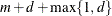 knots as follows. Let
 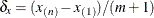 , then interior knots are placed at
![\[ x_{(1)} + j\delta _ x, \quad j=1,\ldots ,m \]](images/statug_glimmix0311.png)
The exterior knots are also evenly spaced with step size
 and start at
  times the machine epsilon. At least one interior knot is required.
- KNOTMIN=number-list
-
provides lower limits for the values of random effects used in the construction of knots for TYPE=RSMOOTH . The items in number-list correspond to the random effects of the radial smooth. If the KNOTMIN= option is not specified, or if the value associated with a particular random effect is set to missing, the minimum is based on the values in the data set for KNOTMETHOD= EQUAL or KNOTMETHOD= KDTREE, and is based on the values in the knot data set for KNOTMETHOD= DATA.
- LDATA=SAS-data-set
-
reads the coefficient matrices
 for the TYPE=LIN(q)
option. You can specify the LDATA= data set in a sparse or dense form. In the sparse form the data set must contain the numeric
variables
for the TYPE=LIN(q)
option. You can specify the LDATA= data set in a sparse or dense form. In the sparse form the data set must contain the numeric
variables Parm,Row,Col, andValue. TheParmvariable contains the indices of the
  matrices. The
 RowandColvariables identify the position within a matrix and theValuevariable contains the matrix element. Values not specified for a particular row and column are set to zero. Missing values are allowed in theValuecolumn of the LDATA= data set; these values are also replaced by zeros. The sparse form is particularly useful if the matrices have only a few nonzero elements.
In the dense form the LDATA= data set contains the numeric variables
ParmandRow(with the same function as above), in addition to the numeric variablesCol1–Colq. If you omit one or more of theCol1–Colq variables from the data set, zeros are assumed for the respective rows and columns of the matrix. Missing values for
 Col1–Colq are ignored in the dense form.The GLIMMIX procedure assumes that the matrices
are symmetric. In the sparse LDATA= form you do not need to specify off-diagonal elements in position  and
and  . One of them is sufficient. Row-column indices are converted in both storage forms into positions in lower triangular storage.
If you specify multiple values in row
. One of them is sufficient. Row-column indices are converted in both storage forms into positions in lower triangular storage.
If you specify multiple values in row  and column
  of a particular matrix, only the last value is used. For example, assume you are specifying elements of a
  matrix. The lower triangular storage of matrix
  defined by
data ldata;
   input parm row col value;
   datalines;
3  2  1  2
3  1  2  5
;
is
![\[ \left[ \begin{array}{llll} 0 & & & \\ 5 & 0 & & \\ 0 & 0 & 0 & \\ 0 & 0 & 0 & 0 \end{array} \right] \]](images/statug_glimmix0323.png)
- NOFULLZ
-
eliminates the columns in
 corresponding to missing levels of
random effects involving CLASS variables. By default, these columns are included in . It is sufficient to specify the NOFULLZ option on any G-side RANDOM statement.
corresponding to missing levels of
random effects involving CLASS variables. By default, these columns are included in . It is sufficient to specify the NOFULLZ option on any G-side RANDOM statement.
-
RESIDUAL
RSIDE -
specifies that the random effects listed in this statement be R-side effects. You use the RESIDUAL option in the RANDOM statement if the nature of the covariance structure requires you to specify an effect. For example, if it is necessary to order the columns of the R-side AR(1) covariance structure by the
timevariable, you can use the RESIDUAL option as in the following statements:class time id; random time / subject=id type=ar(1) residual;
-
SOLUTION
S -
requests that the solution
 for the
random-effects parameters be produced, if the statement defines G-side random effects.
for the
random-effects parameters be produced, if the statement defines G-side random effects.
The numbers displayed in the Std Err Pred column of the "Solution for Random Effects" table are not the standard errors of the
displayed in the Estimate column; rather, they are the square roots of the prediction errors  , where
  is the predictor of the ith random effect and
  is the ith random effect. In pseudo-likelihood methods that are based on linearization, these EBLUPs are the estimated best linear
unbiased predictors in the linear mixed pseudo-model. In models fit by maximum likelihood by using the Laplace approximation
or by using adaptive quadrature, the SOLUTION option displays the empirical Bayes estimates (EBE) of .
is the ith random effect. In pseudo-likelihood methods that are based on linearization, these EBLUPs are the estimated best linear
unbiased predictors in the linear mixed pseudo-model. In models fit by maximum likelihood by using the Laplace approximation
or by using adaptive quadrature, the SOLUTION option displays the empirical Bayes estimates (EBE) of .
-
SUBJECT=effect
SUB=effect -
identifies the subjects in your generalized linear mixed model. Complete independence is assumed across subjects. Specifying a subject effect is equivalent to nesting all other effects in the RANDOM statement within the subject effect.
Continuous variables and computed variables are permitted with the SUBJECT= option. PROC GLIMMIX does not sort by the values of the continuous variable but considers the data to be from a new subject whenever the value of the continuous variable changes from the previous observation. Using a continuous variable can decrease execution time for models with a large number of subjects and also prevents the production of a large "Class Levels Information" table.
- TYPE=covariance-structure
-
specifies the covariance structure of
for G-side effects and
the covariance structure of for R-side effects.
Although a variety of structures are available, many applications call for either simple diagonal (TYPE=VC ) or unstructured covariance matrices. The TYPE=VC (variance components) option is the default structure, and it models a different variance component for each random effect. It is recommended to model unstructured covariance matrices in terms of their Cholesky parameterization (TYPE=CHOL ) rather than TYPE=UN .
If you want different covariance structures in different parts of
, you must use multiple RANDOM statements with different TYPE= options.
Valid values for covariance-structure are as follows. Examples are shown in Table 45.19.
The variances and covariances in the formulas that follow in the TYPE= descriptions are expressed in terms of generic random variables
 and
and  . They represent the G-side random effects or the residual random variables for which the or matrices are constructed.
- ANTE(1)
-
specifies a first-order ante-dependence structure (Kenward 1987; Patel 1991) parameterized in terms of variances and correlation parameters. If t ordered random variables
 have a first-order ante-dependence structure, then each ,
  , is independent of all other
  , given
  . This Markovian structure is characterized by its inverse variance matrix, which is tridiagonal. Parameterizing an ANTE(1)
structure for a random vector of size t requires 2t – 1 parameters: variances
. This Markovian structure is characterized by its inverse variance matrix, which is tridiagonal. Parameterizing an ANTE(1)
structure for a random vector of size t requires 2t – 1 parameters: variances  and t – 1 correlation parameters
  . The covariances among random variables and are then constructed as
![\[ \mr{Cov}\left[\xi _ i,\xi _ j\right] = \sqrt {\sigma ^2_ i\sigma ^2_ j} \, \prod _{k=i}^{j-1}\rho _ k \]](images/statug_glimmix0335.png)
PROC GLIMMIX constrains the correlation parameters to satisfy
 . For variable-order ante-dependence models see Macchiavelli and Arnold (1994).
- AR(1)
-
specifies a first-order autoregressive structure,
![\[ \mr{Cov}\left[\xi _ i,\xi _ j\right] = \sigma ^2 \rho ^{|i^* - j^*|} \]](images/statug_glimmix0337.png)
The values
 and
and  are derived for the ith and jth observations, respectively, and are not necessarily the observation numbers. For example, in the following statements the
values correspond to the class levels for the
are derived for the ith and jth observations, respectively, and are not necessarily the observation numbers. For example, in the following statements the
values correspond to the class levels for the timeeffect of the ith and jth observation within a particular subject:proc glimmix; class time patient; model y = x x*x; random time / sub=patient type=ar(1) residual; run;
PROC GLIMMIX imposes the constraint
 for stationarity.
- ARH(1)
-
specifies a heterogeneous first-order autoregressive structure,
![\[ \mr{Cov}\left[\xi _ i,\xi _ j\right] = \sqrt {\sigma ^2_ i \sigma ^2_ j} \, \rho ^{|i^* - j^*|} \]](images/statug_glimmix0341.png)
with
. This covariance structure has the same correlation pattern as the TYPE=AR(1) structure, but the variances are allowed to
differ.
- ARMA(1,1)
-
specifies the first-order autoregressive moving-average structure,
![\[ \mr{Cov}\left[\xi _ i,\xi _ j\right] = \left\{ \begin{array}{ll} \sigma ^2 & i=j \\ \sigma ^2 \gamma \rho ^{|i^*-j^*|-1} & i \not= j \end{array} \right. \]](images/statug_glimmix0342.png)
Here,
 is the autoregressive parameter,
  models a moving-average component, and
  is a scale parameter. In the notation of Fuller (1976, p. 68),
  and
and
![\[ \gamma = \frac{(1 + b_1\theta _1)(\theta _1 + b_1)}{1 + b^2_1 + 2 b_1 \theta _1} \]](images/statug_glimmix0346.png)
The example in Table 45.19 and
 imply that
![\[ b_1 = \frac{\beta - \sqrt {\beta ^2 - 4\alpha ^2}}{2\alpha } \]](images/statug_glimmix0348.png)
where
 and
and 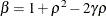 . PROC GLIMMIX imposes the constraints and
  for stationarity, although for some values of and in this region the resulting covariance matrix is not positive definite. When the estimated value of becomes negative, the computed covariance is multiplied by
  to account for the negativity.
- CHOL<(q)>
-
specifies an unstructured variance-covariance matrix parameterized through its Cholesky root. This parameterization ensures that the resulting variance-covariance matrix is at least positive semidefinite. If all diagonal values are nonzero, it is positive definite. For example, a
 unstructured covariance matrix can be written as
![\[ \mr{Var}[\bxi ] = \left[ \begin{array}{cc} \theta _1 & \theta _{12} \\ \theta _{12} & \theta _2 \end{array} \right] \]](images/statug_glimmix0353.png)
Without imposing constraints on the three parameters, there is no guarantee that the estimated variance matrix is positive definite. Even if
 and
and  are nonzero, a large value for
  can lead to a negative eigenvalue of
 ![$\mr{Var}[\bxi ]$](images/statug_glimmix0357.png) . The Cholesky root of a positive definite matrix is a lower triangular matrix
. The Cholesky root of a positive definite matrix is a lower triangular matrix  such that
  . The Cholesky root of the above matrix can be written as
![\[ \mb{C} = \left[ \begin{array}{cc} \alpha _1 & 0 \\ \alpha _{12} & \alpha _2 \end{array} \right] \]](images/statug_glimmix0359.png)
The elements of the unstructured variance matrix are then simply
 ,
,  , and
, and  . Similar operations yield the generalization to covariance matrices of higher orders.
For example, the following statements model the covariance matrix of each subject as an unstructured matrix:
proc glimmix;
   class sub;
   model y = x;
   random _residual_ / subject=sub type=un;
run;
The next set of statements accomplishes the same, but the estimated
matrix is guaranteed to be nonnegative definite:
proc glimmix;
   class sub;
   model y = x;
   random _residual_ / subject=sub type=chol;
run;
The GLIMMIX procedure constrains the diagonal elements of the Cholesky root to be positive. This guarantees a unique solution when the matrix is positive definite.
The optional order parameter
 determines how many bands below the diagonal are modeled. Elements in the lower triangular portion of in bands higher than q are set to zero. If you consider the resulting covariance matrix
  , then the order parameter has the effect of zeroing all off-diagonal elements that are at least q positions away from the diagonal.
Because of its good computational and statistical properties, the Cholesky root parameterization is generally recommended over a completely unstructured covariance matrix (TYPE=UN ). However, it is computationally slightly more involved.
- CS
-
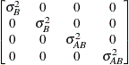
specifies the compound-symmetry structure, which has constant variance and constant covariance
![\[ \mr{Cov}\left[\xi _ i,\xi _ j\right] = \left\{ \begin{array}{lc} \phi + \sigma & i=j \\ \sigma & i \not= j \end{array} \right. \]](images/statug_glimmix0365.png)
The compound symmetry structure arises naturally with nested random effects, such as when subsampling error is nested within experimental error. The models constructed with the following two sets of GLIMMIX statements have the same marginal variance matrix, provided
 is positive:
proc glimmix;
   class block A;
   model y = block A;
   random block*A / type=vc;
run;
proc glimmix;
   class block A;
   model y = block A;
   random _residual_ / subject=block*A
                       type=cs;
run;
In the first case, the
block*Arandom effect models the G-side experimental error. Because the distribution defaults to the normal, the matrix is of form  (see Table 45.20), and
  is the subsampling error variance. The marginal variance for the data from a particular experimental unit is thus
  . This matrix is of compound symmetric form.
Hierarchical random assignments or selections, such as subsampling or split-plot designs, give rise to compound symmetric covariance structures. This implies exchangeability of the observations on the subunit, leading to constant correlations between the observations. Compound symmetric structures are thus usually not appropriate for processes where correlations decline according to some metric, such as spatial and temporal processes.
Note that R-side compound-symmetry structures do not impose any constraint on
. You can thus use an R-side TYPE=CS structure to emulate a variance-component model with unbounded estimate of the variance
component.
- CSH
-
specifies the heterogeneous compound-symmetry structure, which is an equi-correlation structure but allows for different variances
![\[ \mr{Cov}\left[\xi _ i,\xi _ j\right] = \left\{ \begin{array}{lc} \sqrt {\sigma ^2_ i\sigma ^2_ j} & i=j \\ \rho \sqrt {\sigma ^2_ i\sigma ^2_ j} & i \not= j \end{array} \right. \]](images/statug_glimmix0369.png)
- FA(q)
-
specifies the factor-analytic structure with q factors (Jennrich and Schluchter 1986). This structure is of the form
 , where
  is a
is a  rectangular matrix and
  is a
is a  diagonal matrix with t different parameters. When
  , the elements of in its upper-right corner (that is, the elements in the ith row and jth column for
  ) are set to zero to fix the rotation of the structure.
- FA0(q)
-
specifies a factor-analytic structure with q factors of the form
![$\mr{Var}[\bxi ] = \bLambda \bLambda ’$](images/statug_glimmix0377.png) , where is a rectangular matrix and t is the dimension of
, where is a rectangular matrix and t is the dimension of  . When , is a lower triangular matrix. When
  —that is, when the number of factors is less than the dimension of the matrix—this structure is nonnegative definite but not
of full rank. In this situation, you can use it to approximate an unstructured covariance matrix.
—that is, when the number of factors is less than the dimension of the matrix—this structure is nonnegative definite but not
of full rank. In this situation, you can use it to approximate an unstructured covariance matrix.
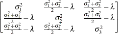
- HF
-
specifies a covariance structure that satisfies the general Huynh-Feldt condition (Huynh and Feldt 1970). For a random vector with t elements, this structure has
 positive parameters and covariances
![\[ \mr{Cov}\left[\xi _ i,\xi _ j\right] = \left\{ \begin{array}{ll} \sigma ^2_ i & i = j \\ 0.5(\sigma ^2_ i+\sigma ^2_ j) - \lambda & i \not= j \end{array} \right. \]](images/statug_glimmix0381.png)
A covariance matrix
 generally satisfies the Huynh-Feldt condition if it can be written as
 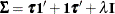 . The preceding parameterization chooses
 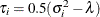 . Several simpler covariance structures give rise to covariance matrices that also satisfy the Huynh-Feldt condition. For
example, TYPE=CS
, TYPE=VC
, and TYPE=UN(1)
are nested within TYPE=HF. You can use the COVTEST
statement to test the HF structure against one of these simpler structures. Note also that the HF structure is nested within
an unstructured covariance matrix.
. Several simpler covariance structures give rise to covariance matrices that also satisfy the Huynh-Feldt condition. For
example, TYPE=CS
, TYPE=VC
, and TYPE=UN(1)
are nested within TYPE=HF. You can use the COVTEST
statement to test the HF structure against one of these simpler structures. Note also that the HF structure is nested within
an unstructured covariance matrix.
The TYPE=HF covariance structure can be sensitive to the choice of starting values and the default MIVQUE(0) starting values can be poor for this structure; you can supply your own starting values with the PARMS statement.
- LIN(q)
-
specifies a general linear covariance structure with q parameters. This structure consists of a linear combination of known matrices that you input with the LDATA= option. Suppose that you want to model the covariance of a random vector of length t, and further suppose that
are symmetric  ) matrices constructed from the information in the LDATA=
data set. Then,
) matrices constructed from the information in the LDATA=
data set. Then,
![\[ \mr{Cov}\left[\xi _ i,\xi _ j\right] = \sum _{k=1}^{q} \theta _ k [\bA _ k]_{ij} \]](images/statug_glimmix0385.png)
where
![$[\bA _ k]_{ij}$](images/statug_glimmix0386.png) denotes the element in row i, column j of matrix
denotes the element in row i, column j of matrix  .
.
Linear structures are very flexible and general. You need to exercise caution to ensure that the variance matrix is positive definite. Note that PROC GLIMMIX does not impose boundary constraints on the parameters
 of a general linear covariance structure. For example, if classification variable
 Ahas 6 levels, the following statements fit a variance component structure for the random effect without boundary constraints:data ldata; retain parm 1 value 1; do row=1 to 6; col=row; output; end; run; proc glimmix data=MyData; class A B; model Y = B; random A / type=lin(1) ldata=ldata; run;
- PSPLINE<(options)>
-
requests that PROC GLIMMIX form a B-spline basis and fits a penalized B-spline (P-spline, Eilers and Marx 1996) with random spline coefficients. This covariance structure is available only for G-side random effects and only a single continuous random effect can be specified with TYPE=PSPLINE. As for TYPE=RSMOOTH, PROC GLIMMIX forms a modified
matrix and fits a mixed model in which the random variables associated with the columns of are independent with a common variance. The matrix is constructed as follows.
Denote as
 the
the  matrix of B-splines of degree d and denote as
  the
the  matrix of rth-order differences. For example, for K = 5,
![\begin{align*} \mb{D}_1 & = \left[ \begin{array}{rrrrr} 1 & -1 & 0 & 0 & 0 \\ 0 & 1 & -1 & 0 & 0 \\ 0 & 0 & 1 & -1 & 0 \\ 0 & 0 & 0 & 1 & -1 \end{array} \right] \\ \mb{D}_2 & = \left[ \begin{array}{rrrrr} 1 & -2 & 1 & 0 & 0 \\ 0 & 1 & -2 & 1 & 0 \\ 0 & 0 & 1 & -2 & 1 \end{array}\right] \\ \mb{D}_3 & = \left[ \begin{array}{rrrrr} 1 & -3 & 3 & -1 & 0 \\ 0 & 1 & -3 & 3 & -1 \end{array} \right] \end{align*}](images/statug_glimmix0393.png)
Then, the
matrix used in fitting the mixed model is the  matrix
![\[ \mb{Z} = \widetilde{\mb{Z}}(\mb{D}_ r’\mb{D}_ r)^-\mb{D}_ r’ \]](images/statug_glimmix0395.png)
The construction of the B-spline knots is controlled with the KNOTMETHOD= EQUAL(m) option and the DEGREE=d suboption of TYPE=PSPLINE. The total number of knots equals the number m of equally spaced interior knots plus d knots at the low end and
 knots at the high end. The number of columns in the B-spline basis equals K = m + d + 1. By default, the interior knots exclude the minimum and maximum of the random-effect values and are based on m – 1 equally spaced intervals. Suppose and are the smallest and largest random-effect values; then interior knots are placed at
![\[ x_{(1)} + j(x_{(n)} - x_{(1)})/(m+1), \quad j=1,\ldots ,m \]](images/statug_glimmix0397.png)
In addition, d evenly spaced exterior knots are placed below
and  exterior knots are placed above
  . The exterior knots are evenly spaced and start at times the machine epsilon. For example, based on the defaults d = 3, r = 3, the following statements lead to 26 total knots and 21 columns in , m = 20, K = m + d + 1 = 24, K – r = 21:
proc glimmix;
   model y = x;
   random x / type=pspline knotmethod=equal(20);
run;
Details about the computation and properties of B-splines can be found in De Boor (2001). You can extend or limit the range of the knots with the KNOTMIN= and KNOTMAX= options. Table 45.18 lists some of the parameters that control this covariance type and their relationships.
Table 45.18: P-Spline Parameters
Parameter
Description
d
Degree of B-spline, default d = 3
r
Order of differencing in construction of
, default r = 3
m
Number of interior knots, default

Total number of knots

Number of columns in B-spline basis

Number of columns in
You can specify the following options for TYPE=PSPLINE:
- DEGREE=d
-
specifies the degree of the B-spline. The default is d = 3.
- DIFFORDER=r
-
specifies the order of the differencing matrix
. The default and maximum is r = 3.
- RSMOOTH<(m | NOLOG)>
-
specifies a radial smoother covariance structure for G-side random effects. This results in an approximate low-rank thin-plate spline where the smoothing parameter is obtained by the estimation method selected with the METHOD= option of the PROC GLIMMIX statement. The smoother is based on the automatic smoother in Ruppert, Wand, and Carroll (2003, Chapter 13.4–13.5), but with a different method of selecting the spline knots. See the section Radial Smoothing Based on Mixed Models for further details about the construction of the smoother and the knot selection.
Radial smoothing is possible in one or more dimensions. A univariate smoother is obtained with a single random effect, while multiple random effects in a RANDOM statement yield a multivariate smoother. Only continuous random effects are permitted with this covariance structure. If
 denotes the number of continuous random effects in the RANDOM statement, then the covariance structure of the random effects
is determined as follows. Suppose that
denotes the number of continuous random effects in the RANDOM statement, then the covariance structure of the random effects
is determined as follows. Suppose that  denotes the vector of random effects for the ith observation. Let
  denote the
  vector of knot coordinates,
  , and K is the total number of knots. The Euclidean distance between the knots is computed as
![\[ d_{kp} = ||\btau _ k - \btau _ p|| = \sqrt {\sum _{j=1}^{n_ r} (\tau _{jk}-\tau _{jp})^2} \]](images/statug_glimmix0408.png)
and the distance between knots and effects is computed as
![\[ h_{ik} = ||\mb{z}_ i - \btau _ k|| = \sqrt {\sum _{j=1}^{n_ r} (z_{ij}-\tau _{jk})^2} \]](images/statug_glimmix0409.png)
The
matrix for the GLMM is constructed as
![\[ \bZ = \widetilde{\bZ }\bOmega ^{-1/2} \]](images/statug_glimmix0410.png)
where the
matrix has typical element
![\[ [\widetilde{\bZ }]_{ik} = \left\{ \begin{array}{ll} h_{ik}^ p & n_ r \, \, \mr{odd} \\ h_{ik}^ p \, \log \{ h_{ik}\} & n_ r \, \, \mr{even} \end{array} \right. \]](images/statug_glimmix0411.png)
and the
 matrix
  has typical element
![\[ [\bOmega ]_{kp} = \left\{ \begin{array}{ll} d_{kp}^ p & n_ r \, \, \mr{odd} \\ d_{kp}^ p \log \{ d_{kp}\} & n_ r \, \, \mr{even} \end{array} \right. \]](images/statug_glimmix0414.png)
The exponent in these expressions equals
 , where the optional value m corresponds to the derivative penalized in the thin-plate spline. A larger value of m will yield a smoother fit. The GLIMMIX procedure requires p > 0 and chooses by default m = 2 if
  and
and  otherwise. The NOLOG option removes the
  and
and  terms from the computation of the and matrices when is even; this yields invariance under rescaling of the coordinates.
Finally, the components of
are assumed to have equal variance  . The "smoothing parameter"
  of the low-rank spline is related to the variance components in the model,
  . See Ruppert, Wand, and Carroll (2003) for details. If the conditional distribution does not provide a scale parameter , you can add a single R-side residual parameter.
The knot selection is controlled with the KNOTMETHOD= option. The GLIMMIX procedure selects knots automatically based on the vertices of a k-d tree or reads knots from a data set that you supply. See the section Radial Smoothing Based on Mixed Models for further details on radial smoothing in the GLIMMIX procedure and its connection to a mixed model formulation.
- SIMPLE
-
- SP(EXP)(c-list)
-
models an exponential spatial or temporal covariance structure, where the covariance between two observations depends on a distance metric
 . The c-list contains the names of the numeric variables used as coordinates to determine distance. For a stochastic process in
  , there are k elements in c-list. If the
  vectors of coordinates for observations i and j are
  and
and  , then PROC GLIMMIX computes the Euclidean distance
![\[ d_{ij} = ||\mb{c}_ i - \mb{c}_ j|| = \sqrt {\sum _{m=1}^{k}(c_{mi} - c_{mj})^2} \]](images/statug_glimmix0426.png)
The covariance between two observations is then
![\[ \mr{Cov}\left[\xi _ i,\xi _ j\right] = \sigma ^2 \exp \{ -d_{ij} / \alpha \} \]](images/statug_glimmix0427.png)
The parameter
 is not what is commonly referred to as the range parameter in geostatistical applications. The practical range of a (second-order
stationary) spatial process is the distance
is not what is commonly referred to as the range parameter in geostatistical applications. The practical range of a (second-order
stationary) spatial process is the distance  at which the correlations fall below 0.05. For the SP(EXP) structure, this distance is
  . PROC GLIMMIX constrains to be positive.
- SP(GAU)(c-list)
-
models a Gaussian covariance structure,
![\[ \mr{Cov}\left[\xi _ i,\xi _ j\right] = \sigma ^2 \exp \{ -d_{ij}^2 / \alpha ^2\} \]](images/statug_glimmix0430.png)
See TYPE=SP(EXP) for the computation of the distance
. The parameter is related to the range of the process as follows. If the practical range is defined as the distance at which the correlations fall below 0.05, then  . PROC GLIMMIX constrains to be positive. See TYPE=SP(EXP) for the computation of the distance from the variables specified in c-list.
- SP(MAT)(c-list)
-
models a covariance structure in the Matérn class of covariance functions (Matérn 1986). The covariance is expressed in the parameterization of Handcock and Stein (1993); Handcock and Wallis (1994); it can be written as
![\[ \mr{Cov}\left[\xi _ i,\xi _ j\right] = \ \sigma ^2\frac{1}{\Gamma (\nu )} \left(\frac{d_{ij}\sqrt {\nu }}{\rho }\right)^{\nu } 2 K_{\nu }\left(\frac{2d_{ij}\sqrt {\nu }}{\rho }\right) \]](images/statug_glimmix0432.png)
The function
 is the modified Bessel function of the second kind of (real) order
  . The smoothness (continuity) of a stochastic process with covariance function in the Matérn class increases with
  . This class thus enables data-driven estimation of the smoothness properties of the process. The covariance is identical
to the exponential model for
. This class thus enables data-driven estimation of the smoothness properties of the process. The covariance is identical
to the exponential model for  (TYPE=SP(EXP)(c-list)), while for
  the model advocated by Whittle (1954) results. As
  , the model approaches the Gaussian covariance structure (TYPE=SP(GAU)(c-list)).
Note that the MIXED procedure offers covariance structures in the Matérn class in two parameterizations, TYPE=SP(MATERN) and TYPE=SP(MATHSW). The TYPE=SP(MAT) in the GLIMMIX procedure is equivalent to TYPE=SP(MATHSW) in the MIXED procedure.
Computation of the function
and its derivatives is numerically demanding; fitting models with Matérn covariance structures can be time-consuming. Good
starting values are essential.
- SP(POW)(c-list)
-
models a power covariance structure,
![\[ \mr{Cov}\left[\xi _ i,\xi _ j\right] = \sigma ^2 \rho ^{d_{ij}} \]](images/statug_glimmix0438.png)
where
 . This is a reparameterization of the exponential structure, TYPE=SP(EXP). Specifically,
  . See TYPE=SP(EXP) for the computation of the distance from the variables specified in c-list. When the estimated value of becomes negative, the computed covariance is multiplied by to account for the negativity.
- SP(POWA)(c-list)
-
models an anisotropic power covariance structure in k dimensions, provided that the coordinate list c-list has k elements. If
 denotes the coordinate for the ith observation of the mth variable in c-list, the covariance between two observations is given by
![\[ \mr{Cov}\left[\xi _ i,\xi _ j\right] = \sigma ^2 \rho _1^{|c_{i1} - c_{j1}|} \rho _2^{|c_{i2} - c_{j2}|} \ldots \rho _ k^{|c_{ik} - c_{jk}|} \]](images/statug_glimmix0442.png)
Note that for k = 1, TYPE=SP(POWA) is equivalent to TYPE=SP(POW), which is itself a reparameterization of TYPE=SP(EXP). When the estimated value of
 becomes negative, the computed covariance is multiplied by
 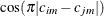 to account for the negativity.
- SP(SPH)(c-list)
-
models a spherical covariance structure,
![\[ \mr{Cov}\left[\xi _ i,\xi _ j\right] = \left\{ \begin{array}{ll} \sigma ^2 \left\{ 1 - \frac{3 d_{ij}}{2 \alpha } + \frac{1}{2} \left(\frac{d_{ij}}{\alpha }\right)^3 \right\} & d_{ij} \leq \alpha \\ 0 & d_{ij} > \alpha \end{array} \right. \]](images/statug_glimmix0445.png)
The spherical covariance structure has a true range parameter. The covariances between observations are exactly zero when their distance exceeds
. See TYPE=SP(EXP) for the computation of the distance from the variables specified in c-list.
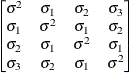
- TOEP
-
models a Toeplitz covariance structure. This structure can be viewed as an autoregressive structure with order equal to the dimension of the matrix,
![\[ \mr{Cov}\left[\xi _ i,\xi _ j\right] = \left\{ \begin{array}{ll} \sigma ^2 & i=j \\ \sigma _{|i-j|} & i \not= j \end{array} \right. \]](images/statug_glimmix0446.png)
- TOEP(q)
-
specifies a banded Toeplitz structure,
![\[ \mr{Cov}\left[\xi _ i,\xi _ j\right] = \left\{ \begin{array}{ll} \sigma ^2 & i=j \\ \sigma _{|i-j|} & |i-j| < q \end{array} \right. \]](images/statug_glimmix0447.png)
This can be viewed as a moving-average structure with order equal to q – 1. The specification TYPE=TOEP(1) is the same as
 , and it can be useful for specifying the same variance component for several effects.
- TOEPH<(q)>
-
models a Toeplitz covariance structure. The correlations of this structure are banded as the TOEP or TOEP(q) structures, but the variances are allowed to vary:
![\[ \mr{Cov}\left[\xi _ i,\xi _ j\right] = \left\{ \begin{array}{ll} \sigma ^2_ i & i = j \\ \rho _{|i-j|} \sqrt {\sigma ^2_ i \sigma ^2_ j} & i \not= j \end{array} \right. \]](images/statug_glimmix0449.png)
The correlation parameters satisfy
 . If you specify the optional value q, the correlation parameters with
  are set to zero, creating a banded correlation structure. The specification TYPE=TOEPH(1) results in a diagonal covariance
matrix with heterogeneous variances.
are set to zero, creating a banded correlation structure. The specification TYPE=TOEPH(1) results in a diagonal covariance
matrix with heterogeneous variances.
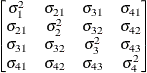
- UN<(q)>
-
specifies a completely general (unstructured) covariance matrix parameterized directly in terms of variances and covariances,
![\[ \mr{Cov}\left[\xi _ i,\xi _ j\right] = \sigma _{ij} \]](images/statug_glimmix0452.png)
The variances are constrained to be nonnegative, and the covariances are unconstrained. This structure is not constrained to be nonnegative definite in order to avoid nonlinear constraints; however, you can use the TYPE=CHOL structure if you want this constraint to be imposed by a Cholesky factorization. If you specify the order parameter q, then PROC GLIMMIX estimates only the first q bands of the matrix, setting elements in all higher bands equal to 0.
- UNR<(q)>
-
specifies a completely general (unstructured) covariance matrix parameterized in terms of variances and correlations,
![\[ \mr{Cov}\left[\xi _ i,\xi _ j\right] = \sigma _ i\sigma _ j\rho _{ij} \]](images/statug_glimmix0453.png)
where
 denotes the standard deviation and the correlation
  is zero when
  and when , provided the order parameter q is given. This structure fits the same model as the TYPE=UN(q) option, but with a different parameterization. The ith variance parameter is
  . The parameter is the correlation between the ith and jth measurements; it satisfies
  . If you specify the order parameter q, then PROC GLIMMIX estimates only the first q bands of the matrix, setting all higher bands equal to zero.
- VC
-
specifies standard variance components and is the default structure for both G-side and R-side covariance structures. In a G-side covariance structure, a distinct variance component is assigned to each effect. In an R-side structure TYPE=VC is usually used only to add overdispersion effects or with the GROUP= option to specify a heterogeneous variance model.
Table 45.19: Covariance Structure Examples
Description
Structure
Example
Variance
ComponentsVC (default)
Compound
Symmetry
Heterogeneous
CS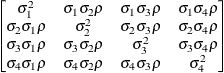
First-Order
Autoregressive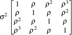
Heterogeneous
AR(1)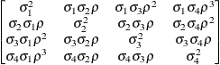
Unstructured
Banded Main
Diagonal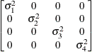
Unstructured
Correlations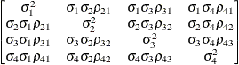
Toeplitz
Toeplitz with
Two Bands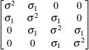
Heterogeneous
Toeplitz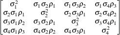
Spatial
Power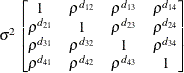
First-Order
Autoregressive
Moving-Average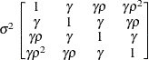
First-Order
Factor
Analytic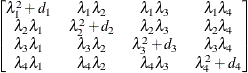
Huynh-Feldt
First-Order
Ante-dependence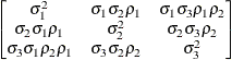
- V<=value-list>
-
requests that blocks of the estimated marginal variance-covariance matrix
 be displayed in generalized linear mixed models. This matrix is based on the last linearization as described in the section
The Pseudo-model. You can use the value-list to select the subjects for which the matrix is displayed. If value-list is not specified, the
be displayed in generalized linear mixed models. This matrix is based on the last linearization as described in the section
The Pseudo-model. You can use the value-list to select the subjects for which the matrix is displayed. If value-list is not specified, the  matrix for the first subject is chosen.
Note that the value-list refers to subjects as the processing units in the "Dimensions" table. For example, the following statements request that the estimated marginal variance matrix for the second subject be displayed:
proc glimmix;
   class A B;
   model y = B;
   random int / subject=A;
   random int / subject=A*B v=2;
run;
The subject effect for processing in this case is the
Aeffect, because it is contained in theA*Binteraction. If there is only a single subject as per the "Dimensions" table, then the V option displays an matrix.
See the section Processing by Subjects for how the GLIMMIX procedure determines the number of subjects in the "Dimensions" table.
The GLIMMIX procedure displays blanks for values that are 0.
- VC<=value-list>
-
displays the lower-triangular Cholesky root of the blocks of the estimated
matrix. See the V
option for the specification of value-list.
- VCI<=value-list>
-
displays the inverse Cholesky root of the blocks of the estimated
matrix. See the V
option for the specification of value-list.
- VCORR<=value-list>
-
displays the correlation matrix corresponding to the blocks of the estimated
matrix. See the V
option for the specification of value-list.
- VI<=value-list>
-
displays the inverse of the blocks of the estimated
matrix. See the V
option for the specification of value-list.
-
WEIGHT<=variable>
WT<=variable> -
specifies a variable to be used as the weight for the units at the current level in a weighted multilevel model. If a weight variable is not specified in the WEIGHT option, a weight of 1 is used. For details on the use of weights in multilevel models, see the section Pseudo-likelihood Estimation for Weighted Multilevel Models.