The GLIMMIX Procedure
-
Overview

-
Getting Started
-
SyntaxPROC GLIMMIX StatementBY StatementCLASS StatementCODE StatementCONTRAST StatementCOVTEST StatementEFFECT StatementESTIMATE StatementFREQ StatementID StatementLSMEANS StatementLSMESTIMATE StatementMODEL StatementNLOPTIONS StatementOUTPUT StatementPARMS StatementRANDOM StatementSLICE StatementSTORE StatementWEIGHT StatementProgramming StatementsUser-Defined Link or Variance Function
-
DetailsGeneralized Linear Models TheoryGeneralized Linear Mixed Models TheoryGLM Mode or GLMM ModeStatistical Inference for Covariance ParametersDegrees of Freedom MethodsEmpirical Covariance ("Sandwich") EstimatorsExploring and Comparing Covariance MatricesProcessing by SubjectsRadial Smoothing Based on Mixed ModelsOdds and Odds Ratio EstimationParameterization of Generalized Linear Mixed ModelsResponse-Level Ordering and ReferencingComparing the GLIMMIX and MIXED ProceduresSingly or Doubly Iterative FittingDefault Estimation TechniquesDefault OutputNotes on Output StatisticsODS Table NamesODS Graphics
-
ExamplesBinomial Counts in Randomized BlocksMating Experiment with Crossed Random EffectsSmoothing Disease Rates; Standardized Mortality RatiosQuasi-likelihood Estimation for Proportions with Unknown DistributionJoint Modeling of Binary and Count DataRadial Smoothing of Repeated Measures DataIsotonic Contrasts for Ordered AlternativesAdjusted Covariance Matrices of Fixed EffectsTesting Equality of Covariance and Correlation MatricesMultiple Trends Correspond to Multiple Extrema in Profile LikelihoodsMaximum Likelihood in Proportional Odds Model with Random EffectsFitting a Marginal (GEE-Type) ModelResponse Surface Comparisons with Multiplicity AdjustmentsGeneralized Poisson Mixed Model for Overdispersed Count DataComparing Multiple B-SplinesDiallel Experiment with Multimember Random EffectsLinear Inference Based on Summary DataWeighted Multilevel Model for Survey DataQuadrature Method for Multilevel Model
- References
Example 45.15 Comparing Multiple B-Splines
This example uses simulated data to demonstrate the use of the nonpositional syntax (see the section Positional and Nonpositional Syntax for Contrast Coefficients for details) in combination with the experimental EFFECT
statement to produce interesting predictions and comparisons in models containing fixed spline effects. Consider the data
in the following DATA step. Each of the 100 observations for the continuous response variable y is associated with one of two groups.
data spline;
   input group y @@;
   x = _n_;
   datalines;
 1    -.020 1    0.199 2    -1.36 1    -.026
 2    -.397 1    0.065 2    -.861 1    0.251
 1    0.253 2    -.460 2    0.195 2    -.108
 1    0.379 1    0.971 1    0.712 2    0.811
 2    0.574 2    0.755 1    0.316 2    0.961
 2    1.088 2    0.607 2    0.959 1    0.653
 1    0.629 2    1.237 2    0.734 2    0.299
 2    1.002 2    1.201 1    1.520 1    1.105
 1    1.329 1    1.580 2    1.098 1    1.613
 2    1.052 2    1.108 2    1.257 2    2.005
 2    1.726 2    1.179 2    1.338 1    1.707
 2    2.105 2    1.828 2    1.368 1    2.252
 1    1.984 2    1.867 1    2.771 1    2.052
 2    1.522 2    2.200 1    2.562 1    2.517
 1    2.769 1    2.534 2    1.969 1    2.460
 1    2.873 1    2.678 1    3.135 2    1.705
 1    2.893 1    3.023 1    3.050 2    2.273
 2    2.549 1    2.836 2    2.375 2    1.841
 1    3.727 1    3.806 1    3.269 1    3.533
 1    2.948 2    1.954 2    2.326 2    2.017
 1    3.744 2    2.431 2    2.040 1    3.995
 2    1.996 2    2.028 2    2.321 2    2.479
 2    2.337 1    4.516 2    2.326 2    2.144
 2    2.474 2    2.221 1    4.867 2    2.453
 1    5.253 2    3.024 2    2.403 1    5.498
;
The following statements produce a scatter plot of the response variable by group (Output 45.15.1):
proc sgplot data=spline;
   scatter y=y x=x / group=group name="data";
   keylegend "data"  / title="Group";
run;
Output 45.15.1: Scatter Plot of Observed Data by Group
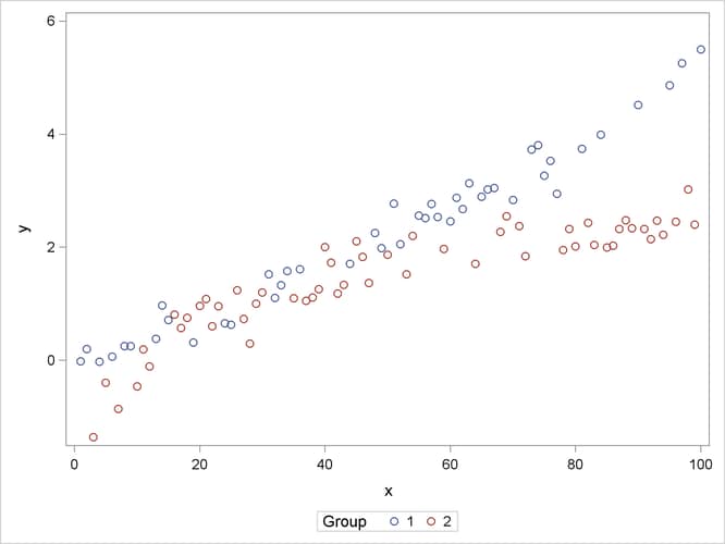
The trends in the two groups exhibit curvature, but the type of curvature is not the same in the groups. Also, there appear
to be ranges of x values where the groups are similar and areas where the point scatters separate. To model the trends in the two groups separately
and with flexibility, you might want to allow for some smooth trends in x that vary by group. Consider the following PROC GLIMMIX statements:
proc glimmix data=spline outdesign=x;
   class group;
   effect spl = spline(x);
   model y = group spl*group / s noint;
   output out=gmxout pred=p;
run;
The EFFECT
statement defines a constructed effect named spl by expanding the x into a spline with seven columns. The group main effect creates separate intercepts for the groups, and the interaction of the group variable with the spline effect creates separate trends. The NOINT
option suppresses the intercept. This is not necessary and is done here only for convenience of interpretation. The OUTPUT
statement computes predicted values.
The "Parameter Estimates" table contains the estimates of the group-specific "intercepts," the spline coefficients varied by group, and the residual variance ("Scale," Output 45.15.2).
Output 45.15.2: Parameter Estimates in Two-Group Spline Model
| Parameter Estimates | |||||||
|---|---|---|---|---|---|---|---|
| Effect | spl | group | Estimate | Standard Error |
DF | t Value | Pr > |t| |
| group | 1 | 9.7027 | 3.1342 | 86 | 3.10 | 0.0026 | |
| group | 2 | 6.3062 | 2.6299 | 86 | 2.40 | 0.0187 | |
| spl*group | 1 | 1 | -11.1786 | 3.7008 | 86 | -3.02 | 0.0033 |
| spl*group | 1 | 2 | -20.1946 | 3.9765 | 86 | -5.08 | <.0001 |
| spl*group | 2 | 1 | -9.5327 | 3.2576 | 86 | -2.93 | 0.0044 |
| spl*group | 2 | 2 | -5.8565 | 2.7906 | 86 | -2.10 | 0.0388 |
| spl*group | 3 | 1 | -8.9612 | 3.0718 | 86 | -2.92 | 0.0045 |
| spl*group | 3 | 2 | -5.5567 | 2.5717 | 86 | -2.16 | 0.0335 |
| spl*group | 4 | 1 | -7.2615 | 3.2437 | 86 | -2.24 | 0.0278 |
| spl*group | 4 | 2 | -4.3678 | 2.7247 | 86 | -1.60 | 0.1126 |
| spl*group | 5 | 1 | -6.4462 | 2.9617 | 86 | -2.18 | 0.0323 |
| spl*group | 5 | 2 | -4.0380 | 2.4589 | 86 | -1.64 | 0.1042 |
| spl*group | 6 | 1 | -4.6382 | 3.7095 | 86 | -1.25 | 0.2146 |
| spl*group | 6 | 2 | -4.3029 | 3.0479 | 86 | -1.41 | 0.1616 |
| spl*group | 7 | 1 | 0 | . | . | . | . |
| spl*group | 7 | 2 | 0 | . | . | . | . |
| Scale | 0.07352 | 0.01121 | . | . | . | ||
Because the B-spline coefficients for an observation sum to 1 and the model contains group-specific constants, the last spline coefficient in each group is zero. In other words, you can achieve exactly the same fit with the MODEL statement
model y = spl*group / noint;
or
model y = spl*group;
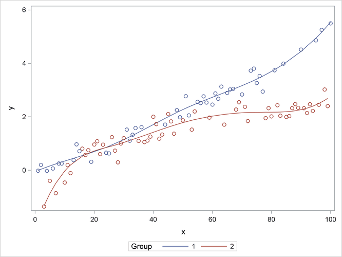
The following statements graph the observed and fitted values in the two groups (Output 45.15.3):
proc sgplot data=gmxout;
   series  y=p x=x / group=group name="fit";
   scatter y=y x=x / group=group;
   keylegend "fit" / title="Group";
run;
Output 45.15.3: Observed and Predicted Values by Group
Suppose that you are interested in estimating the mean response at particular values of x and in performing comparisons of predicted values. The following program uses ESTIMATE
statements with nonpositional syntax to accomplish this:
proc glimmix data=spline;
   class group;
   effect spl = spline(x);
   model y = group spl*group / s noint;
   estimate 'Group 1, x=20' group 1    group*spl [1,1 20] / e;
   estimate 'Group 2, x=20' group 0  1 group*spl [1,2 20];
   estimate 'Diff at x=20 ' group 1 -1 group*spl [1,1 20] [-1,2 20];
run;
The first ESTIMATE
statement predicts the mean response at x = 20 in group 1. The E
option requests the coefficient vector for this linear combination of the parameter estimates. The coefficient for the group effect is entered with positional (standard) syntax. The coefficients for the group*spl effect are formed based on nonpositional syntax. Because this effect comprises the interaction of a standard effect (group) with a constructed effect, the values and levels for the standard effect must precede those for the constructed effect.
A similar statement produces the predicted mean at x = 20 in group 2.
The GLIMMIX procedure interprets the syntax
group*spl [1,2 20]
as follows: construct the spline basis at x = 20 as appropriate for group 2; then multiply the resulting coefficients for these columns of the  matrix with 1.
The final ESTIMATE statement represents the difference between the predicted values; it is a group comparison at x = 20.
Output 45.15.4: Coefficients from First ESTIMATE Statement
| Coefficients for Estimate Group 1, x=20 |
|||
|---|---|---|---|
| Effect | spl | group | Row1 |
| group | 1 | 1 | |
| group | 2 | ||
| spl*group | 1 | 1 | 0.0021 |
| spl*group | 1 | 2 | |
| spl*group | 2 | 1 | 0.3035 |
| spl*group | 2 | 2 | |
| spl*group | 3 | 1 | 0.619 |
| spl*group | 3 | 2 | |
| spl*group | 4 | 1 | 0.0754 |
| spl*group | 4 | 2 | |
| spl*group | 5 | 1 | |
| spl*group | 5 | 2 | |
| spl*group | 6 | 1 | |
| spl*group | 6 | 2 | |
| spl*group | 7 | 1 | |
| spl*group | 7 | 2 | |
The "Coefficients" table shows how the value 20 supplied in the ESTIMATE statement was expanded into the appropriate spline basis (Output 45.15.4). There is no significant difference between the group means at x = 20 (p = 0.8346, Output 45.15.5).
Output 45.15.5: Results from ESTIMATE Statements
The group comparisons you can achieve in this way are comparable to slices of interaction effects with classification effects.
There are, however, no preset number of levels at which to perform the comparisons because x is continuous. If you add further x values for the comparisons, a multiplicity correction is in order to control the familywise Type I error. The following statements
compare the groups at values  and compute simulation-based step-down-adjusted p-values. The results appear in Output 45.15.6. (The numeric results for simulation-based p-value adjustments depend slightly on the value of the random number seed.)
ods select Estimates;
proc glimmix data=spline;
   class group;
   effect spl = spline(x);
   model y = group spl*group / s;
   estimate 'Diff at x= 0' group 1 -1 group*spl [1,1  0] [-1,2  0],
            'Diff at x= 5' group 1 -1 group*spl [1,1  5] [-1,2  5],
            'Diff at x=10' group 1 -1 group*spl [1,1 10] [-1,2 10],
            'Diff at x=15' group 1 -1 group*spl [1,1 15] [-1,2 15],
            'Diff at x=20' group 1 -1 group*spl [1,1 20] [-1,2 20],
            'Diff at x=25' group 1 -1 group*spl [1,1 25] [-1,2 25],
            'Diff at x=30' group 1 -1 group*spl [1,1 30] [-1,2 30],
            'Diff at x=35' group 1 -1 group*spl [1,1 35] [-1,2 35],
            'Diff at x=40' group 1 -1 group*spl [1,1 40] [-1,2 40],
            'Diff at x=45' group 1 -1 group*spl [1,1 45] [-1,2 45],
            'Diff at x=50' group 1 -1 group*spl [1,1 50] [-1,2 50],
            'Diff at x=55' group 1 -1 group*spl [1,1 55] [-1,2 55],
            'Diff at x=60' group 1 -1 group*spl [1,1 60] [-1,2 60],
            'Diff at x=65' group 1 -1 group*spl [1,1 65] [-1,2 65],
            'Diff at x=70' group 1 -1 group*spl [1,1 70] [-1,2 70],
            'Diff at x=75' group 1 -1 group*spl [1,1 75] [-1,2 75],
            'Diff at x=80' group 1 -1 group*spl [1,1 80] [-1,2 80] /
            adjust=sim(seed=1) stepdown;
run;
Output 45.15.6: Estimates with Multiplicity Adjustments
| Estimates Adjustment for Multiplicity: Holm-Simulated |
||||||
|---|---|---|---|---|---|---|
| Label | Estimate | Standard Error |
DF | t Value | Pr > |t| | Adj P |
| Diff at x= 0 | 12.4124 | 4.2130 | 86 | 2.95 | 0.0041 | 0.0210 |
| Diff at x= 5 | 1.0376 | 0.1759 | 86 | 5.90 | <.0001 | <.0001 |
| Diff at x=10 | 0.3778 | 0.1540 | 86 | 2.45 | 0.0162 | 0.0554 |
| Diff at x=15 | 0.05822 | 0.1481 | 86 | 0.39 | 0.6952 | 0.9043 |
| Diff at x=20 | -0.02602 | 0.1243 | 86 | -0.21 | 0.8346 | 0.9578 |
| Diff at x=25 | 0.02014 | 0.1312 | 86 | 0.15 | 0.8783 | 0.9578 |
| Diff at x=30 | 0.1023 | 0.1378 | 86 | 0.74 | 0.4600 | 0.7419 |
| Diff at x=35 | 0.1924 | 0.1236 | 86 | 1.56 | 0.1231 | 0.2890 |
| Diff at x=40 | 0.2883 | 0.1114 | 86 | 2.59 | 0.0113 | 0.0465 |
| Diff at x=45 | 0.3877 | 0.1195 | 86 | 3.24 | 0.0017 | 0.0098 |
| Diff at x=50 | 0.4885 | 0.1308 | 86 | 3.74 | 0.0003 | 0.0022 |
| Diff at x=55 | 0.5903 | 0.1231 | 86 | 4.79 | <.0001 | <.0001 |
| Diff at x=60 | 0.7031 | 0.1125 | 86 | 6.25 | <.0001 | <.0001 |
| Diff at x=65 | 0.8401 | 0.1203 | 86 | 6.99 | <.0001 | <.0001 |
| Diff at x=70 | 1.0147 | 0.1348 | 86 | 7.52 | <.0001 | <.0001 |
| Diff at x=75 | 1.2400 | 0.1326 | 86 | 9.35 | <.0001 | <.0001 |
| Diff at x=80 | 1.5237 | 0.1281 | 86 | 11.89 | <.0001 | <.0001 |
There are significant differences at the low end and high end of the x range. Notice that without the multiplicity adjustment you would have concluded at the 0.05 level that the groups are significantly
different at x = 10. At the 0.05 level, the groups separate significantly for  and
and  .
.