The GLIMMIX Procedure
-
Overview

-
Getting Started
-
SyntaxPROC GLIMMIX StatementBY StatementCLASS StatementCODE StatementCONTRAST StatementCOVTEST StatementEFFECT StatementESTIMATE StatementFREQ StatementID StatementLSMEANS StatementLSMESTIMATE StatementMODEL StatementNLOPTIONS StatementOUTPUT StatementPARMS StatementRANDOM StatementSLICE StatementSTORE StatementWEIGHT StatementProgramming StatementsUser-Defined Link or Variance Function
-
DetailsGeneralized Linear Models TheoryGeneralized Linear Mixed Models TheoryGLM Mode or GLMM ModeStatistical Inference for Covariance ParametersDegrees of Freedom MethodsEmpirical Covariance ("Sandwich") EstimatorsExploring and Comparing Covariance MatricesProcessing by SubjectsRadial Smoothing Based on Mixed ModelsOdds and Odds Ratio EstimationParameterization of Generalized Linear Mixed ModelsResponse-Level Ordering and ReferencingComparing the GLIMMIX and MIXED ProceduresSingly or Doubly Iterative FittingDefault Estimation TechniquesDefault OutputNotes on Output StatisticsODS Table NamesODS Graphics
-
ExamplesBinomial Counts in Randomized BlocksMating Experiment with Crossed Random EffectsSmoothing Disease Rates; Standardized Mortality RatiosQuasi-likelihood Estimation for Proportions with Unknown DistributionJoint Modeling of Binary and Count DataRadial Smoothing of Repeated Measures DataIsotonic Contrasts for Ordered AlternativesAdjusted Covariance Matrices of Fixed EffectsTesting Equality of Covariance and Correlation MatricesMultiple Trends Correspond to Multiple Extrema in Profile LikelihoodsMaximum Likelihood in Proportional Odds Model with Random EffectsFitting a Marginal (GEE-Type) ModelResponse Surface Comparisons with Multiplicity AdjustmentsGeneralized Poisson Mixed Model for Overdispersed Count DataComparing Multiple B-SplinesDiallel Experiment with Multimember Random EffectsLinear Inference Based on Summary DataWeighted Multilevel Model for Survey DataQuadrature Method for Multilevel Model
- References
Example 45.9 Testing Equality of Covariance and Correlation Matrices
Fisher’s iris data are widely used in multivariate statistics. They comprise measurements in millimeters of four flower attributes, the length and width of sepals and petals for 50 specimens from each of three species, Iris setosa, I. versicolor, and I. virginica (Fisher 1936).
When modeling multiple attributes from the same specimen, correlations among measurements from the same flower must be taken into account. Unstructured covariance matrices are common in this multivariate setting. Species comparisons can focus on comparisons of mean response, but comparisons of the variation and covariation are also of interest. In this example, the equivalence of covariance and correlation matrices among the species are examined.
The iris data set is available in the Sashelp library. The following step displays the first 10 observations of the iris data in multivariate format—that is, each observation contains multiple response variables. The DATA step that follows creates
a data set in univariate form, where each observation corresponds to a single response variable. This is the form needed by
the GLIMMIX procedure.
proc print data=Sashelp.iris(obs=10);
run;
Output 45.9.1: Fisher (1936) Iris Data
data iris_univ;
   set sashelp.iris;
   retain id 0;
   array y (4) SepalLength SepalWidth PetalLength PetalWidth;
   id+1;
   do var=1 to 4;
      response = y{var};
      output;
   end;
   drop SepalLength SepalWidth PetalLength PetalWidth:;
run;
The following GLIMMIX statements fit a model with separate unstructured covariance matrices for each species:
ods select FitStatistics CovParms CovTests;
proc glimmix data=iris_univ;
   class species var id;
   model response = species*var;
   random _residual_ / type=un group=species subject=id;
   covtest homogeneity;
run;
The mean function is modeled as a cell-means model that allows for different means for each species and outcome variable.
The covariances are modeled directly (R-side) rather than through random effects. The ID variable identifies the individual plant, so that responses from different plants are independent. The GROUP=
SPECIES option varies the parameters of the unstructured covariance matrix by species. Hence, this model has 30 covariance
parameters: 10 unique parameters for a  covariance matrix for each of three species.
The COVTEST statement requests a test of homogeneity—that is, it tests whether varying the covariance parameters by the group effect provides a significantly better fit compared to a model in which different groups share the same parameter.
Output 45.9.2: Fit Statistics for Analysis of Fisher’s Iris Data
The "Fit Statistics" table shows the –2 restricted (residual) log likelihood in the full model and other fit statistics (Output 45.9.2). The "-2 Res Log Likelihood" sets the benchmark against which a model with homogeneity constraint is compared. Output 45.9.3 displays the 30 covariance parameters in this model.
There appear to be substantial differences among the covariance parameters from different groups. For example, the residual variability of the petal length of the three species is 12.4249, 26.6433, and 40.4343, respectively. The homogeneity hypothesis restricts these variances to be equal and similarly for the other covariance parameters. The results from the COVTEST statement are shown in Output 45.9.4.
Output 45.9.3: Covariance Parameters Varied by Species (TYPE=UN)
| Covariance Parameter Estimates | ||||
|---|---|---|---|---|
| Cov Parm | Subject | Group | Estimate | Standard Error |
| UN(1,1) | id | Species Setosa | 12.4249 | 2.5102 |
| UN(2,1) | id | Species Setosa | 9.9216 | 2.3775 |
| UN(2,2) | id | Species Setosa | 14.3690 | 2.9030 |
| UN(3,1) | id | Species Setosa | 1.6355 | 0.9052 |
| UN(3,2) | id | Species Setosa | 1.1698 | 0.9552 |
| UN(3,3) | id | Species Setosa | 3.0159 | 0.6093 |
| UN(4,1) | id | Species Setosa | 1.0331 | 0.5508 |
| UN(4,2) | id | Species Setosa | 0.9298 | 0.5859 |
| UN(4,3) | id | Species Setosa | 0.6069 | 0.2755 |
| UN(4,4) | id | Species Setosa | 1.1106 | 0.2244 |
| UN(1,1) | id | Species Versicolor | 26.6433 | 5.3828 |
| UN(2,1) | id | Species Versicolor | 8.5184 | 2.6144 |
| UN(2,2) | id | Species Versicolor | 9.8469 | 1.9894 |
| UN(3,1) | id | Species Versicolor | 18.2898 | 4.3398 |
| UN(3,2) | id | Species Versicolor | 8.2653 | 2.4149 |
| UN(3,3) | id | Species Versicolor | 22.0816 | 4.4612 |
| UN(4,1) | id | Species Versicolor | 5.5780 | 1.6617 |
| UN(4,2) | id | Species Versicolor | 4.1204 | 1.0641 |
| UN(4,3) | id | Species Versicolor | 7.3102 | 1.6891 |
| UN(4,4) | id | Species Versicolor | 3.9106 | 0.7901 |
| UN(1,1) | id | Species Virginica | 40.4343 | 8.1690 |
| UN(2,1) | id | Species Virginica | 9.3763 | 3.2213 |
| UN(2,2) | id | Species Virginica | 10.4004 | 2.1012 |
| UN(3,1) | id | Species Virginica | 30.3290 | 6.6262 |
| UN(3,2) | id | Species Virginica | 7.1380 | 2.7395 |
| UN(3,3) | id | Species Virginica | 30.4588 | 6.1536 |
| UN(4,1) | id | Species Virginica | 4.9094 | 2.5916 |
| UN(4,2) | id | Species Virginica | 4.7629 | 1.4367 |
| UN(4,3) | id | Species Virginica | 4.8824 | 2.2750 |
| UN(4,4) | id | Species Virginica | 7.5433 | 1.5240 |
Output 45.9.4: Likelihood Ratio Test of Homogeneity
Denote as  the covariance matrix for species
  with elements
  . In processing the COVTEST
hypothesis
. In processing the COVTEST
hypothesis  , the GLIMMIX procedure fits a model that satisfies the constraints
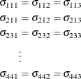
where is the covariance between the ith and jth variable for the kth species. The –2 restricted log likelihood of this restricted model is 2959.55 (Output 45.9.4). The change of 146.66 compared to the full model is highly significant. There is sufficient evidence to reject the notion
of equal covariance matrices among the three iris species.
Equality of covariance matrices implies equality of correlation matrices, but the reverse is not true. Fewer constraints are needed to equate correlations because the diagonal entries of the covariance matrices are free to vary. In order to test the equality of the correlation matrices among the three species, you can parameterize the unstructured covariance matrix in terms of the correlations and use a COVTEST statement with general contrasts, as shown in the following statements:
ods select FitStatistics CovParms CovTests;
proc glimmix data=iris_univ;
   class species var id;
   model response = species*var;
   random _residual_ / type=unr group=species subject=id;
   covtest 'Equal Covariance Matrices'  homogeneity;
   covtest 'Equal Correlation Matrices' general
        0  0  0  0  1  0  0  0  0  0
        0  0  0  0 -1  0  0  0  0  0,
        0  0  0  0  1  0  0  0  0  0
        0  0  0  0  0  0  0  0  0  0
        0  0  0  0 -1  0  0  0  0  0,
        0  0  0  0  0  1  0  0  0  0
        0  0  0  0  0 -1  0  0  0  0,
        0  0  0  0  0  1  0  0  0  0
        0  0  0  0  0  0  0  0  0  0
        0  0  0  0  0 -1  0  0  0  0,
        0  0  0  0  0  0  1  0  0  0
        0  0  0  0  0  0 -1  0  0  0,
        0  0  0  0  0  0  1  0  0  0
        0  0  0  0  0  0  0  0  0  0
        0  0  0  0  0  0 -1  0  0  0,
        0  0  0  0  0  0  0  1  0  0
        0  0  0  0  0  0  0 -1  0  0,
        0  0  0  0  0  0  0  1  0  0
        0  0  0  0  0  0  0  0  0  0
        0  0  0  0  0  0  0 -1  0  0,
        0  0  0  0  0  0  0  0  1  0
        0  0  0  0  0  0  0  0 -1  0,
        0  0  0  0  0  0  0  0  1  0
        0  0  0  0  0  0  0  0  0  0
        0  0  0  0  0  0  0  0  -1 0,
        0  0  0  0  0  0  0  0  0  1
        0  0  0  0  0  0  0  0  0 -1,
        0  0  0  0  0  0  0  0  0  1
        0  0  0  0  0  0  0  0  0  0
        0  0  0  0  0  0  0  0  0 -1 / estimates;
run;
The TYPE=UNR
structure is a reparameterization of TYPE=UN
. The models provide the same fit, as seen by comparison of the "Fit Statistics" tables in Output 45.9.2 and Output 45.9.5. The covariance parameters are ordered differently, however. In each group, the four variances precede the six correlations
(Output 45.9.5). The first COVTEST
statement tests the homogeneity hypothesis in terms of the UNR parameterization, and the result is identical to the test
in Output 45.9.4. The second COVTEST
statement restricts the correlations to be equal across groups. If  is the correlation between the ith and jth variable for the kth species, the 12 restrictions are
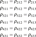
The ESTIMATES option in the COVTEST statement requests that the GLIMMIX procedure display the covariance parameter estimates in the restricted model (Output 45.9.5).
Output 45.9.5: Fit Statistics, Covariance Parameters (TYPE=UNR), and Likelihood Ratio Tests for Equality of Covariance and Correlation Matrices
| Covariance Parameter Estimates | ||||
|---|---|---|---|---|
| Cov Parm | Subject | Group | Estimate | Standard Error |
| Var(1) | id | Species Setosa | 12.4249 | 2.5102 |
| Var(2) | id | Species Setosa | 14.3690 | 2.9030 |
| Var(3) | id | Species Setosa | 3.0159 | 0.6093 |
| Var(4) | id | Species Setosa | 1.1106 | 0.2244 |
| Corr(2,1) | id | Species Setosa | 0.7425 | 0.06409 |
| Corr(3,1) | id | Species Setosa | 0.2672 | 0.1327 |
| Corr(3,2) | id | Species Setosa | 0.1777 | 0.1383 |
| Corr(4,1) | id | Species Setosa | 0.2781 | 0.1318 |
| Corr(4,2) | id | Species Setosa | 0.2328 | 0.1351 |
| Corr(4,3) | id | Species Setosa | 0.3316 | 0.1271 |
| Var(1) | id | Species Versicolor | 26.6433 | 5.3828 |
| Var(2) | id | Species Versicolor | 9.8469 | 1.9894 |
| Var(3) | id | Species Versicolor | 22.0816 | 4.4612 |
| Var(4) | id | Species Versicolor | 3.9106 | 0.7901 |
| Corr(2,1) | id | Species Versicolor | 0.5259 | 0.1033 |
| Corr(3,1) | id | Species Versicolor | 0.7540 | 0.06163 |
| Corr(3,2) | id | Species Versicolor | 0.5605 | 0.09797 |
| Corr(4,1) | id | Species Versicolor | 0.5465 | 0.1002 |
| Corr(4,2) | id | Species Versicolor | 0.6640 | 0.07987 |
| Corr(4,3) | id | Species Versicolor | 0.7867 | 0.05445 |
| Var(1) | id | Species Virginica | 40.4343 | 8.1690 |
| Var(2) | id | Species Virginica | 10.4004 | 2.1012 |
| Var(3) | id | Species Virginica | 30.4588 | 6.1536 |
| Var(4) | id | Species Virginica | 7.5433 | 1.5240 |
| Corr(2,1) | id | Species Virginica | 0.4572 | 0.1130 |
| Corr(3,1) | id | Species Virginica | 0.8642 | 0.03616 |
| Corr(3,2) | id | Species Virginica | 0.4010 | 0.1199 |
| Corr(4,1) | id | Species Virginica | 0.2811 | 0.1316 |
| Corr(4,2) | id | Species Virginica | 0.5377 | 0.1015 |
| Corr(4,3) | id | Species Virginica | 0.3221 | 0.1280 |
| Tests of Covariance Parameters Based on the Restricted Likelihood |
|||||||||||||||||||||||||||||||||||
|---|---|---|---|---|---|---|---|---|---|---|---|---|---|---|---|---|---|---|---|---|---|---|---|---|---|---|---|---|---|---|---|---|---|---|---|
| Label | DF | -2 Res Log Like | ChiSq | Pr > ChiSq | Estimates H0 | Note | |||||||||||||||||||||||||||||
| Est1 | Est2 | Est3 | Est4 | Est5 | Est6 | Est7 | Est8 | Est9 | Est10 | Est11 | Est12 | Est13 | Est14 | Est15 | Est16 | Est17 | Est18 | Est19 | Est20 | Est21 | Est22 | Est23 | Est24 | Est25 | Est26 | Est27 | Est28 | Est29 | Est30 | ||||||
| Equal Covariance Matrices | 20 | 2959.55 | 146.66 | <.0001 | 26.5004 | 11.5395 | 18.5179 | 4.1883 | 0.5302 | 0.7562 | 0.3779 | 0.3645 | 0.4705 | 0.4845 | 26.5004 | 11.5395 | 18.5179 | 4.1883 | 0.5302 | 0.7562 | 0.3779 | 0.3645 | 0.4705 | 0.4845 | 26.5004 | 11.5395 | 18.5179 | 4.1883 | 0.5302 | 0.7562 | 0.3779 | 0.3645 | 0.4705 | 0.4845 | DF |
| Equal Correlation Matrices | 12 | 2876.38 | 63.49 | <.0001 | 16.4715 | 14.8656 | 4.8427 | 1.4392 | 0.5612 | 0.6827 | 0.4016 | 0.3844 | 0.4976 | 0.5219 | 24.4020 | 9.1566 | 17.4434 | 3.0021 | 0.5612 | 0.6827 | 0.4016 | 0.3844 | 0.4976 | 0.5219 | 35.0544 | 10.8350 | 27.3593 | 8.1395 | 0.5612 | 0.6827 | 0.4016 | 0.3844 | 0.4976 | 0.5219 | DF |
| DF: P-value based on a chi-square with DF degrees of freedom. |
The result of the homogeneity test is identical to that in Output 45.9.4. The hypothesis of equality of the correlation matrices is also rejected with a chi-square value of 63.49 and a p-value of  . Notice, however, that the chi-square statistic is smaller than in the test of homogeneity due to the smaller number of restrictions
imposed on the full model. The estimate of the common correlation matrix in the restricted model is
. Notice, however, that the chi-square statistic is smaller than in the test of homogeneity due to the smaller number of restrictions
imposed on the full model. The estimate of the common correlation matrix in the restricted model is
![\[ \left[ \begin{array}{llll} 1 & 0.561 & 0.683 & 0.384 \\ 0.561 & 1 & 0.402 & 0.498 \\ 0.683 & 0.402 & 1 & 0.522 \\ 0.384 & 0.498 & 0.522 & 1 \end{array} \right] \]](images/statug_glimmix1043.png)