The GLIMMIX Procedure

COVTEST Statement

Subsections:

Test Specification
Covariance Test Options

COVTEST <'label'> <test-specification> </ options>;

The COVTEST statement provides a mechanism to obtain statistical inferences for the covariance parameters. Significance tests are based on the ratio of (residual) likelihoods or pseudo-likelihoods. Confidence limits and bounds are computed as Wald or likelihood ratio limits. You can specify multiple COVTEST statements.

The likelihood ratio test is obtained by fitting the model subject to the constraints imposed by the test-specification. The test statistic is formed as twice the difference of the (possibly restricted) log (pseudo-) likelihoods of the full and the reduced models. Note that fitting the null model does not necessarily require fewer computer resources compared to fitting the full model. The optimization settings for refitting the model are the same as for the full model and can be controlled with the NLOPTIONS statement.

Common questions in mixed modeling are whether variance components are zero, whether random effects are independent, and whether rows (columns) can be added or removed from an unstructured covariance matrix. When the parameters under the null hypothesis fall on the boundary of the parameter space, the distribution of the likelihood ratio statistic can be a complicated mixture of distributions. In certain situations it is known to be a relatively straightforward mixture of central chi-square distributions. When the GLIMMIX procedure recognizes the model and hypothesis as a case for which the mixture is readily available, the p-value of the likelihood ratio test is determined accordingly as a linear combination of central chi-square probabilities. The Note column in the "Likelihood Ratio Tests for Covariance Parameters" table along with the table’s footnotes informs you about when mixture distributions are used in the calculation of p-values. You can find important statistical and computational details about likelihood ratio testing of covariance parameters with the GLIMMIX procedure in the section Statistical Inference for Covariance Parameters.

In generalized linear mixed models that depend on pseudo-data, the GLIMMIX procedure fits the null model for a test of covariance parameters to the final pseudo-data of the converged optimization.

Table 45.6 summarizes the options available in the COVTEST statement.

Table 45.6: COVTEST Statement Options

Option	Description
Test specification
TESTDATA=	Reads in covariance parameter values from a SAS data set
GENERAL	Provides a general facility to test linear combinations of covariance parameters
Covariance Test Options
CL	Requests confidence limits for the covariance parameter estimates
CLASSICAL	Computes the likelihood ratio test p-value using the classical method
DF=	Specifies the degrees of freedom
ESTIMATES	Displays the estimates of the covariance parameters under the null hypothesis
MAXITER=	Limits the number of iterations
PARMS	Displays the values of the covariance parameters under the null hypothesis
RESTART	Specifies that starting values for the covariance parameters
TOLERANCE=	Sets the tolerance level of the parameter space boundary
WALD	Produces Wald Z tests
WGHT=	Supplies weights for the computation of p-values

Test Specification

The test-specification in the COVTEST statement draws on keywords that represent a particular null hypothesis, lists or data sets of parameter values, or general contrast specifications. Valid keywords are as follows:

GLM | INDEP

tests the model against a null model of complete independence. All G-side covariance parameters are eliminated and the R-side covariance structure is reduced to a diagonal structure.

DIAGG

tests for a diagonal G matrix by constraining off-diagonal elements in G to zero. The R-side structure is not modified.

DIAGR | CINDEP

tests for conditional independence by reducing the R-side covariance structure to diagonal form. The G-side structure is not modified.

HOMOGENEITY

tests homogeneity of covariance parameters across groups by imposing equality constraints. For example, the following statements fit a one-way model with heterogeneous variances and test whether the model could be reduced to a one-way analysis with the same variance across groups:

proc glimmix;
   class A;
   model y = a;
   random _residual_ / group=A;
   covtest 'common variance' homogeneity;
run;

See Example 45.9 for an application with groups and unstructured covariance matrices.

START | INITIAL

compares the final estimates to the starting values of the covariance parameter estimates. This option is useful, for example, if you supply starting values in the PARMS statement and want to test whether the optimization produced significantly better values. In GLMMs based on pseudo-data, the likelihoods that use the starting and the final values are based on the final pseudo-data.

ZEROG

tests whether the G matrix can be reduced to a zero matrix. This eliminates all G-side random effects from the model.

Only a single keyword is permitted in the COVTEST statement. To test more complicated hypotheses, you can formulate tests with the following specifications.

TESTDATA=data-set TDATA=data-set

reads in covariance parameter values from a SAS data set. The data set should contain the numerical variable Estimate or numerical variables named Covpi. The GLIMMIX procedure associates the values for Covpi with the ith covariance parameter.

For data sets containing the numerical variable Estimate, the GLIMMIX procedure fixes the ith covariance parameter value at the value of the ith observation in the data set. A missing value indicates not to fix the particular parameter. PROC GLIMMIX performs one likelihood ratio test for the TESTDATA= data set.

For data sets containing numerical variables named Covpi, the procedure performs one likelihood ratio test for each observation in the TESTDATA= data set. You do not have to specify a Covpi variable for every covariance parameter. If the value for the variable is not missing, PROC GLIMMIX fixes the associated covariance parameter in the null model. Consider the following statements:

data TestDataSet;
   input covp1 covp2 covp3;
   datalines;
. 0 .
0 0 .
. 0 0
0 0 0
;

proc glimmix method=mspl;
   class subject x;
   model y = x age x*age;
   random intercept age / sub=subject type=un;
   covtest testdata=TestDataSet;
run;

Because the $\bG$ matrix is a $(2 \times 2)$ unstructured matrix, the first observation of the TestDataSet corresponds to zeroing the covariance between the random intercept and the random slope. When the reduced model is fit, the variances of the intercept and slope are reestimated. The second observation reduces the model to one with only a random slope in age. The third reduces the model to a random intercept model. The last observation eliminates the $\bG$ matrix altogether.

Note that the tests associated with the first and last set of covariance parameters in TestDataSet can also be obtained by using keywords:

proc glimmix;
   class subject x;
   model y = x age x*age;
   random intercept age / sub=subject type=un;
   covtest DiagG;
   covtest GLM;
run;

value-list

supplies a list of values at which to fix the covariance parameters. A missing value in the list indicates that the covariance parameter is not fixed. If the list is shorter than the number of covariance parameters, missing values are assumed for all parameters not specified. The COVTEST statements that test the random intercept and random slope in the previous example are as follows:

proc glimmix;
   class subject x;
   model y = x age x*age;
   random intercept age / sub=subject type=un;
   covtest 0 0;
   covtest . 0 0;
run;

GENERAL coefficients <,coefficients> <,…> CONTRAST coefficients <,coefficients> <,…>

provides a general facility to test linear combinations of covariance parameters. You can specify one or more sets of coefficients. The position of a coefficient in the list corresponds to the position of the parameter in the "Covariance Parameter Estimates" table. The linear combination of covariance parameters that is implied by each set of coefficients is tested against zero. If the list of coefficients is shorter than the number of covariance parameters, a zero coefficient is assumed for the remaining parameters.

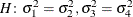For example, in a heterogeneous variance model with four groups, the following statements test the simultaneous hypothesis $H\colon \sigma ^2_1 = \sigma ^2_2, \sigma ^2_3 = \sigma ^2_4$ :

proc glimmix;
   class A;
   model y = a;
   random _residual_ / group=A;
   covtest 'pair-wise homogeneity'
           general  1 -1  0  0,
                    0  0  1 -1;
run;

In a repeated measures study with four observations per subject, the COVTEST statement in the following example tests whether the four correlation parameters are identical:

proc glimmix;
   class subject drug time;
   model y = drug time drug*time;
   random _residual_ / sub=subject type=unr;
   covtest 'Homogeneous correlation'
        general  0 0 0 0 1 -1            ,
                 0 0 0 0 1  0 -1         ,
                 0 0 0 0 1  0  0 -1      ,
                 0 0 0 0 1  0  0  0 -1   ,
                 0 0 0 0 1  0  0  0  0 -1;
run;

Notice that the variances (the first four covariance parameters) are allowed to vary. The null model for this test is thus a heterogeneous compound symmetry model.

The degrees of freedom associated with these general linear hypotheses are determined as the rank of the matrix $\bL \bL ’$ , where $\mb{L}$ is the $k \times q$ matrix of coefficients and q is the number of covariance parameters. Notice that the coefficients in a row do not have to sum to zero. The following statement tests $H\colon \theta _1 = 3\theta _2, \, \theta _3 = 0$ :

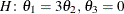covtest general 1 -3, 0 0 1;

Covariance Test Options

You can specify the following options in the COVTEST statement after a slash (/).

CL<(suboptions)>

requests confidence limits or bounds for the covariance parameter estimates. These limits are displayed as extra columns in the "Covariance Parameter Estimates" table.

The following suboptions determine the computation of confidence bounds and intervals. See the section Statistical Inference for Covariance Parameters for details about constructing likelihood ratio confidence limits for covariance parameters with PROC GLIMMIX.

ALPHA=number

determines the confidence level for constructing confidence limits for the covariance parameters. The value of number must be between 0 and 1, the default is 0.05, and the confidence level is 1 – number.

LOWERBOUND LOWER

requests lower confidence bounds.

TYPE=method

determines how the GLIMMIX procedure constructs confidence limits for covariance parameters. The valid methods are PLR (or PROFILE), ELR (or ESTIMATED), and WALD. TYPE=PLR (TYPE=PROFILE) requests confidence bounds by inversion of the profile (restricted) likelihood ratio (PLR). If $\theta$ is the parameter of interest, L denotes the likelihood (possibly restricted and possibly a pseudo-likelihood), and $\btheta _2$ is the vector of the remaining (nuisance) parameters, then the profile likelihood is defined as

$L(\btheta _2|\widetilde{\theta }) = \sup _{\btheta _2} L(\widetilde{\theta },\btheta _2)$

for a given value $\widetilde{\theta }$ of $\theta$ . If $L(\widehat{\btheta })$ is the overall likelihood evaluated at the estimates $\widehat{\btheta }$ , the $(1-\alpha )\times 100\%$ confidence region for $\theta$ satisfies the inequality

$2 \left\{ L(\widehat{\btheta }) - L(\btheta _2|\widetilde{\theta }) \right\} \leq \chi ^2_{1,(1-\alpha )}$

where $\chi ^2_{1,(1-\alpha )}$ is the cutoff from a chi-square distribution with one degree of freedom and $\alpha$ probability to its right. If a residual scale parameter $\phi$ is profiled from the estimation, and $\theta$ is expressed in terms of a ratio with $\phi$ during estimation, then profile likelihood confidence limits are constructed for the ratio of the parameter with the residual variance. A column showing the ratio estimates is added to the "Covariance Parameter Estimates" table in this case. To obtain profile likelihood ratio limits for the parameters, rather than their ratios, and for the residual variance, use the NOPROFILE option in the PROC GLIMMIX statement. Also note that METHOD= LAPLACE or METHOD= QUAD implies the NOPROFILE option.

The TYPE=ELR (TYPE=ESTIMATED) option constructs bounds from the estimated likelihood (Pawitan 2001), where nuisance parameters are held fixed at the (restricted) maximum (pseudo-) likelihood estimates of the model. Estimated likelihood intervals are computationally less demanding than profile likelihood intervals, but they do not take into account the variability of the nuisance parameters or the dependence among the covariance parameters. See the section Statistical Inference for Covariance Parameters for a geometric interpretation and comparison of ELR versus PLR confidence bounds. A $(1-\alpha )\times 100\%$ confidence region based on the estimated likelihood is defined by the inequality

$2 \left\{ L(\widehat{\btheta }) - L(\widetilde{\theta },\widehat{\btheta }_2) \right\} \leq \chi ^2_{1,(1-\alpha )}$

where $L(\widetilde{\theta },\widehat{\btheta }_2)$ is the likelihood evaluated at $\widetilde{\theta }$ and the component of $\widehat{\btheta }$ that corresponds to $\btheta _2$ . Estimated likelihood ratio intervals tend to perform well when the correlations between the parameter of interest and the nuisance parameters is small. Their coverage probabilities can fall short of the nominal coverage otherwise. You can display the correlation matrix of the covariance parameter estimates with the ASYCORR option in the PROC GLIMMIX statement.

If you choose TYPE=PLR or TYPE=ELR, the GLIMMIX procedure reports the right-tail probability of the associated single-degree-of-freedom likelihood ratio test along with the confidence bounds. This helps you diagnose whether solutions to the inequality could be found. If the reported probability exceeds $\alpha$ , the associated bound does not meet the inequality. This might occur, for example, when the parameter space is bounded and the likelihood at the boundary values has not dropped by a sufficient amount to satisfy the test inequality.

The TYPE=WALD method requests confidence limits based on the Wald-type statistic $Z_\theta = \widehat{\theta }/ \mr{ease}(\widehat{\theta })$ , where $\mr{ease}$ is the estimated asymptotic standard error of the covariance parameter. For parameters that have a lower boundary constraint of zero, a Satterthwaite approximation is used to construct limits of the form

$\frac{\nu \widehat{\theta }}{\chi ^2_{\nu ,1-\alpha /2}} \leq \theta \leq \frac{\nu \widehat{\theta }}{\chi ^2_{\nu ,\alpha /2}}$

where $\nu = 2Z^2$ , and the denominators are quantiles of the $\chi ^2$ distribution with $\nu$ degrees of freedom. See Milliken and Johnson (1992) and Burdick and Graybill (1992) for similar techniques. For all other parameters, Wald Z-scores and normal quantiles are used to construct the limits. Such limits are also provided for variance components if you specify the NOBOUND option in the PROC GLIMMIX statement or the PARMS statement.

UPPERBOUND UPPER

requests upper confidence bounds.

If you do not specify any suboptions, the default is to compute two-sided Wald confidence intervals with confidence level $1 - \alpha = 0.95$ .

CLASSICAL

requests that the p-value of the likelihood ratio test be computed by the classical method. If $\widehat{\lambda }$ is the realized value of the test statistic in the likelihood ratio test,

$p = \mr{Pr} \left(\chi ^2_\nu \geq \widehat{\lambda }\right)$

where $\nu$ is the degrees of freedom of the hypothesis.

DF=value-list

enables you to supply degrees of freedom $\nu _1, \ldots , \nu _ k$ for the computation of p-values from chi-square mixtures. The mixture weights $w_1, \ldots , w_ k$ are supplied with the WGHT= option. If no weights are specified, an equal weight distribution is assumed. If $\widehat{\lambda }$ is the realized value of the test statistic in the likelihood ratio test, PROC GLIMMIX computes the p-value as (Shapiro 1988)

$p = \sum _{i=1}^{k} w_ i \mr{Pr} \left(\chi ^2_{\nu _ i} \geq \widehat{\lambda } \right)$

Note that $\chi ^2_0 \equiv 0$ and that mixture weights are scaled to sum to one. If you specify more weights than degrees of freedom in value-list, the rank of the hypothesis (DF column) is substituted for the missing degrees of freedom.

Specifying a single value $\nu$ for value-list without giving mixture weights is equivalent to computing the p-value as

$p = \mr{Pr} \left(\chi ^2_\nu \geq \widehat{\lambda }\right)$

For example, the following statements compute the p-value based on a chi-square distribution with one degree of freedom:

proc glimmix noprofile;
   class A sub;
   model score = A;
   random _residual_ / type=ar(1) subject=sub;
   covtest 'ELR low' 30.62555 0.7133361 / df=1;
run;

The DF column of the COVTEST output will continue to read 2 regardless of the DF= specification, however, because the DF column reflects the rank of the hypothesis and equals the number of constraints imposed on the full model.

ESTIMATES EST

displays the estimates of the covariance parameters under the null hypothesis. Specifying the ESTIMATES option in one COVTEST statement has the same effect as specifying the option in every COVTEST statement.

MAXITER=number

limits the number of iterations when you are refitting the model under the null hypothesis to number iterations. If the null model does not converge before the limit is reached, no p-values are produced.

PARMS

displays the values of the covariance parameters under the null hypothesis. This option is useful if you supply multiple sets of parameter values with the TESTDATA= option. Specifying the PARMS option in one COVTEST statement has the same effect as specifying the option in every COVTEST statement.

RESTART

specifies that starting values for the covariance parameters for the null model are obtained by the same mechanism as starting values for the full models. For example, if you do not specify a PARMS statement, the RESTART option computes MIVQUE(0) estimates under the null model (Goodnight 1978a). If you provide starting values with the PARMS statement, the starting values for the null model are obtained by applying restrictions to the starting values for the full model.

By default, PROC GLIMMIX obtains starting values by applying null model restrictions to the converged estimates of the full model. Although this is computationally expedient, the method does not always lead to good starting values for the null model, depending on the nature of the model and hypothesis. In particular, when you receive a warning about parameters not specified under $H_0$ falling on the boundary, the RESTART option can be useful.

TOLERANCE=r

Values within tolerance $r \geq 0$ of the boundary of the parameter space are considered on the boundary when PROC GLIMMIX examines estimates of nuisance parameters under $H_0$ and determines whether mixture weights and degrees of freedom can be obtained. In certain cases, when parameters not specified under the null hypothesis are on boundaries, the asymptotic distribution of the likelihood ratio statistic is not a mixture of chi-squares (see, for example, case 8 in Self and Liang 1987). The default for r is 1E4 times the machine epsilon; this product is approximately 1E–12 on most computers.

WALD

produces Wald Z tests for the covariance parameters based on the estimates and asymptotic standard errors in the "Covariance Parameter Estimates" table.

WGHT=value-list

enables you to supply weights for the computation of p-values from chi-square mixtures. See the DF= option for details. Mixture weights are scaled to sum to one.