The GLIMMIX Procedure
-
Overview

-
Getting Started
-
SyntaxPROC GLIMMIX StatementBY StatementCLASS StatementCODE StatementCONTRAST StatementCOVTEST StatementEFFECT StatementESTIMATE StatementFREQ StatementID StatementLSMEANS StatementLSMESTIMATE StatementMODEL StatementNLOPTIONS StatementOUTPUT StatementPARMS StatementRANDOM StatementSLICE StatementSTORE StatementWEIGHT StatementProgramming StatementsUser-Defined Link or Variance Function
-
DetailsGeneralized Linear Models TheoryGeneralized Linear Mixed Models TheoryGLM Mode or GLMM ModeStatistical Inference for Covariance ParametersDegrees of Freedom MethodsEmpirical Covariance ("Sandwich") EstimatorsExploring and Comparing Covariance MatricesProcessing by SubjectsRadial Smoothing Based on Mixed ModelsOdds and Odds Ratio EstimationParameterization of Generalized Linear Mixed ModelsResponse-Level Ordering and ReferencingComparing the GLIMMIX and MIXED ProceduresSingly or Doubly Iterative FittingDefault Estimation TechniquesDefault OutputNotes on Output StatisticsODS Table NamesODS Graphics
-
ExamplesBinomial Counts in Randomized BlocksMating Experiment with Crossed Random EffectsSmoothing Disease Rates; Standardized Mortality RatiosQuasi-likelihood Estimation for Proportions with Unknown DistributionJoint Modeling of Binary and Count DataRadial Smoothing of Repeated Measures DataIsotonic Contrasts for Ordered AlternativesAdjusted Covariance Matrices of Fixed EffectsTesting Equality of Covariance and Correlation MatricesMultiple Trends Correspond to Multiple Extrema in Profile LikelihoodsMaximum Likelihood in Proportional Odds Model with Random EffectsFitting a Marginal (GEE-Type) ModelResponse Surface Comparisons with Multiplicity AdjustmentsGeneralized Poisson Mixed Model for Overdispersed Count DataComparing Multiple B-SplinesDiallel Experiment with Multimember Random EffectsLinear Inference Based on Summary DataWeighted Multilevel Model for Survey DataQuadrature Method for Multilevel Model
- References
Example 45.2 Mating Experiment with Crossed Random Effects
McCullagh and Nelder (1989, Ch. 14.5) describe a mating experiment—conducted by S. Arnold and P. Verell at the University of Chicago, Department of Ecology and Evolution—involving two geographically isolated populations of mountain dusky salamanders. One goal of the experiment was to determine whether barriers to interbreeding have evolved in light of the geographical isolation of the populations. In this case, matings within a population should be more successful than matings between the populations. The experiment conducted in the summer of 1986 involved 40 animals, 20 rough butt (R) and 20 whiteside (W) salamanders, with equal numbers of males and females. The animals were grouped into two sets of R males, two sets of R females, two sets of W males, and two sets of W females, so that each set comprised five salamanders. Each set was mated against one rough butt and one whiteside set, creating eight crossings. Within the pairings of sets, each female was paired to three male animals. The salamander mating data have been used by a number of authors; see, for example, McCullagh and Nelder (1989); Schall (1991); Karim and Zeger (1992); Breslow and Clayton (1993); Wolfinger and O’Connell (1993); Shun (1997).
The following DATA step creates the data set for the analysis.
data salamander;
   input day fpop$ fnum mpop$ mnum mating @@;
   datalines;
4  rb  1 rb  1 1  4  rb  2 rb  5 1
4  rb  3 rb  2 1  4  rb  4 rb  4 1
4  rb  5 rb  3 1  4  rb  6 ws  9 1
4  rb  7 ws  8 0  4  rb  8 ws  6 0
4  rb  9 ws 10 0  4  rb 10 ws  7 0
4  ws  1 rb  9 0  4  ws  2 rb  7 0
4  ws  3 rb  8 0  4  ws  4 rb 10 0
4  ws  5 rb  6 0  4  ws  6 ws  5 0
4  ws  7 ws  4 1  4  ws  8 ws  1 1
4  ws  9 ws  3 1  4  ws 10 ws  2 1
8  rb  1 ws  4 1  8  rb  2 ws  5 1
8  rb  3 ws  1 0  8  rb  4 ws  2 1
8  rb  5 ws  3 1  8  rb  6 rb  9 1
8  rb  7 rb  8 0  8  rb  8 rb  6 1
8  rb  9 rb  7 0  8  rb 10 rb 10 0
8  ws  1 ws  9 1  8  ws  2 ws  6 0
8  ws  3 ws  7 0  8  ws  4 ws 10 1
8  ws  5 ws  8 1  8  ws  6 rb  2 0
8  ws  7 rb  1 1  8  ws  8 rb  4 0
8  ws  9 rb  3 1  8  ws 10 rb  5 0
12 rb  1 rb  5 1  12 rb  2 rb  3 1
12 rb  3 rb  1 1  12 rb  4 rb  2 1
12 rb  5 rb  4 1  12 rb  6 ws 10 1
12 rb  7 ws  9 0  12 rb  8 ws  7 0
12 rb  9 ws  8 1  12 rb 10 ws  6 1
12 ws  1 rb  7 1  12 ws  2 rb  9 0
12 ws  3 rb  6 0  12 ws  4 rb  8 1
12 ws  5 rb 10 0  12 ws  6 ws  3 1
12 ws  7 ws  5 1  12 ws  8 ws  2 1
12 ws  9 ws  1 1  12 ws 10 ws  4 0
16 rb  1 ws  1 0  16 rb  2 ws  3 1
16 rb  3 ws  4 1  16 rb  4 ws  5 0
16 rb  5 ws  2 1  16 rb  6 rb  7 0
16 rb  7 rb  9 1  16 rb  8 rb 10 0
16 rb  9 rb  6 1  16 rb 10 rb  8 0
16 ws  1 ws 10 1  16 ws  2 ws  7 1
16 ws  3 ws  9 0  16 ws  4 ws  8 1
16 ws  5 ws  6 0  16 ws  6 rb  4 0
16 ws  7 rb  2 0  16 ws  8 rb  5 0
16 ws  9 rb  1 1  16 ws 10 rb  3 1
20 rb  1 rb  4 1  20 rb  2 rb  1 1
20 rb  3 rb  3 1  20 rb  4 rb  5 1
20 rb  5 rb  2 1  20 rb  6 ws  6 1
20 rb  7 ws  7 0  20 rb  8 ws 10 1
20 rb  9 ws  9 1  20 rb 10 ws  8 1
20 ws  1 rb 10 0  20 ws  2 rb  6 0
20 ws  3 rb  7 0  20 ws  4 rb  9 0
20 ws  5 rb  8 0  20 ws  6 ws  2 0
20 ws  7 ws  1 1  20 ws  8 ws  5 1
20 ws  9 ws  4 1  20 ws 10 ws  3 1
24 rb  1 ws  5 1  24 rb  2 ws  2 1
24 rb  3 ws  3 1  24 rb  4 ws  4 1
24 rb  5 ws  1 1  24 rb  6 rb  8 1
24 rb  7 rb  6 0  24 rb  8 rb  9 1
24 rb  9 rb 10 1  24 rb 10 rb  7 0
24 ws  1 ws  8 1  24 ws  2 ws 10 0
24 ws  3 ws  6 1  24 ws  4 ws  9 1
24 ws  5 ws  7 0  24 ws  6 rb  1 0
24 ws  7 rb  5 1  24 ws  8 rb  3 0
24 ws  9 rb  4 0  24 ws 10 rb  2 0
;
The first observation, for example, indicates that rough butt female 1 was paired in the laboratory on day 4 of the experiment with rough butt male 1, and the pair mated. On the same day rough butt female 7 was paired with whiteside male 8, but the pairing did not result in mating of the animals.
The model adopted by many authors for these data comprises fixed effects for gender and population, their interaction, and
male and female random effects. Specifically, let  ,
,  ,
,  , and
, and  denote the mating probabilities between the populations, where the first subscript identifies the female partner of the pair.
Then, you model
denote the mating probabilities between the populations, where the first subscript identifies the female partner of the pair.
Then, you model
![\[ \log \left\{ \frac{\pi _{kl}}{1-\pi _{kl}} \right\} = \tau _{kl} + \gamma _ f + \gamma _ m \quad k,l \in \{ R,W\} \]](images/statug_glimmix0987.png)
where  and
and  are independent random variables representing female and male random effects (20 each), and
  denotes the average logit of mating between females of population k and males of population l. The following statements fit this model by pseudo-likelihood:
proc glimmix data=salamander;
   class fpop fnum mpop mnum;
   model mating(event='1') = fpop|mpop / dist=binary;
   random fpop*fnum mpop*mnum;
   lsmeans fpop*mpop / ilink;
run;
The response variable is the two-level variable mating. Because it is coded as zeros and ones, and because PROC GLIMMIX models by default the probability of the first level according
to the response-level ordering, the EVENT=’1’ option instructs PROC GLIMMIX to model the probability of a successful mating.
The distribution of the mating variable, conditional on the random effects, is binary.
The fpop*fnum effect in the RANDOM
statement creates a random intercept for each female animal. Because fpop and fnum are CLASS
variables, the effect has 20 levels (10 rb and 10 ws females). Similarly, the mpop*mnum effect creates the random intercepts for the male animals. Because no TYPE=
is specified in the RANDOM
statement, the covariance structure defaults to TYPE=VC
. The random effects and their levels are independent, and each effect has its own variance component. Because the conditional
distribution of the data, conditioned on the random effects, is binary, no
extra scale parameter ( ) is added.
The LSMEANS
statement requests least squares means for the four levels of the fpop*mpop effect, which are estimates of the cell means in the  classification of female and male populations. The ILINK
option in the LSMEANS
statement requests that the estimated means and standard errors are also reported on the scale of the data. This yields estimates
of the four mating probabilities, , , , and .
classification of female and male populations. The ILINK
option in the LSMEANS
statement requests that the estimated means and standard errors are also reported on the scale of the data. This yields estimates
of the four mating probabilities, , , , and .
The "Model Information" table displays general information about the model being fit (Output 45.2.1).
Output 45.2.1: Analysis of Mating Experiment with Crossed Random Effects
The response variable mating follows a binary distribution (conditional on the random effects). Hence, the mean of the data is an event probability,  , and the logit of this probability is linearly related to the linear predictor of the model. The variance function is the
default function that is implied by the distribution,
, and the logit of this probability is linearly related to the linear predictor of the model. The variance function is the
default function that is implied by the distribution,  . The variance matrix is not blocked, because the GLIMMIX procedure does not process the data by subjects (see the section
Processing by Subjects for details). The estimation technique is the default method for GLMMs, residual pseudo-likelihood (METHOD=
RSPL), and degrees of freedom for tests and confidence intervals are determined by the containment method.
. The variance matrix is not blocked, because the GLIMMIX procedure does not process the data by subjects (see the section
Processing by Subjects for details). The estimation technique is the default method for GLMMs, residual pseudo-likelihood (METHOD=
RSPL), and degrees of freedom for tests and confidence intervals are determined by the containment method.
The "Class Level Information" table in Output 45.2.2 lists the levels of the variables listed in the CLASS statement, as well as the order of the levels.
Output 45.2.2: Class Level Information and Number of Observations
Note that there are two female populations and two male populations; also, the variables fnum and mnum have 10 levels each. As a consequence, the effects fpop*fnum and mpop*mnum identify the 20 females and males, respectively. The effect fpop*mpop identifies the four mating types.
The "Response Profile Table," which is displayed for binary or multinomial data, lists the levels of the response variable and their order (Output 45.2.3). With binary data, the table also provides information about which level of the response variable defines the event. Because of the EVENT=’1’ response variable option in the MODEL statement, the probability being modeled is that of the higher-ordered value.
Output 45.2.3: Response Profiles
There are two covariance parameters in this model, the variance of the fpop*fnum effect and the variance of the mpop*mnum effect (Output 45.2.4). Both parameters are modeled as G-side parameters. The nine columns in the  matrix comprise the intercept, two columns each for the levels of the
 fpop and mpop effects, and four columns for their interaction. The  matrix has 40 columns, one for each animal. Because the data are not processed by subjects, PROC GLIMMIX assumes the data
consist of a single subject (a single block in
matrix has 40 columns, one for each animal. Because the data are not processed by subjects, PROC GLIMMIX assumes the data
consist of a single subject (a single block in  ).
).
Output 45.2.4: Model Dimensions Information
The "Optimization Information" table displays basic information about the optimization (Output 45.2.5). The default technique for GLMMs is the quasi-Newton method. There are two parameters in the optimization, which correspond to the two variance components. The 17 fixed effects parameters are not part of the optimization. The initial optimization computes pseudo-data based on the response values in the data set rather than from estimates of a generalized linear model fit.
Output 45.2.5: Optimization Information
The GLIMMIX procedure performs eight optimizations after the initial optimization (Output 45.2.6). That is, following the initial pseudo-data creation, the pseudo-data were updated eight more times and a total of nine linear mixed models were estimated.
Output 45.2.6: Iteration History and Convergence Status
| Iteration History | |||||
|---|---|---|---|---|---|
| Iteration | Restarts | Subiterations | Objective Function |
Change | Max Gradient |
| 0 | 0 | 4 | 537.09173501 | 2.00000000 | 1.719E-8 |
| 1 | 0 | 3 | 544.12516903 | 0.66319780 | 1.14E-8 |
| 2 | 0 | 2 | 545.89139118 | 0.13539318 | 1.609E-6 |
| 3 | 0 | 2 | 546.10489538 | 0.01742065 | 5.89E-10 |
| 4 | 0 | 1 | 546.13075146 | 0.00212475 | 9.654E-7 |
| 5 | 0 | 1 | 546.13374731 | 0.00025072 | 1.346E-8 |
| 6 | 0 | 1 | 546.13409761 | 0.00002931 | 1.84E-10 |
| 7 | 0 | 0 | 546.13413861 | 0.00000000 | 4.285E-6 |
The "Covariance Parameter Estimates" table lists the estimates for the two variance components and their estimated standard errors (Output 45.2.7). The heterogeneity (in the logit of the mating probabilities) among the females is considerably larger than the heterogeneity among the males.
Output 45.2.7: Estimated Covariance Parameters and Approximate Standard Errors
The "Type III Tests of Fixed Effects" table indicates a significant interaction between the male and female populations (Output 45.2.8). A comparison in the logits of mating success in pairs with R females and W females depends on whether the male partner in the pair is the same species. The "fpop*mpop Least Squares Means" table shows this effect more clearly (Output 45.2.9).
Output 45.2.8: Tests of Main Effects and Interaction
Output 45.2.9: Interaction Least Squares Means
| fpop*mpop Least Squares Means | ||||||||
|---|---|---|---|---|---|---|---|---|
| fpop | mpop | Estimate | Standard Error |
DF | t Value | Pr > |t| | Mean | Standard Error Mean |
| rb | rb | 1.1629 | 0.5961 | 81 | 1.95 | 0.0545 | 0.7619 | 0.1081 |
| rb | ws | 0.7839 | 0.5729 | 81 | 1.37 | 0.1750 | 0.6865 | 0.1233 |
| ws | rb | -1.4119 | 0.6143 | 81 | -2.30 | 0.0241 | 0.1959 | 0.09678 |
| ws | ws | 1.0151 | 0.5871 | 81 | 1.73 | 0.0876 | 0.7340 | 0.1146 |
In a pairing with a male rough butt salamander, the logit drops sharply from 1.1629 to –1.4119 when the male is paired with
a whiteside female instead of a female from its own population. The corresponding estimated probabilities of mating success
are  and
and  . If the same comparisons are made in pairs with whiteside males, then you also notice a drop in the logit if the female comes
from a different population, 1.0151 versus 0.7839. The change is considerably less, though, corresponding to mating probabilities
of
. If the same comparisons are made in pairs with whiteside males, then you also notice a drop in the logit if the female comes
from a different population, 1.0151 versus 0.7839. The change is considerably less, though, corresponding to mating probabilities
of  and
and  . Whiteside females appear to be successful with their own population. Whiteside males appear to succeed equally well with
female partners of the two populations.
. Whiteside females appear to be successful with their own population. Whiteside males appear to succeed equally well with
female partners of the two populations.
This insight into the factor-level comparisons can be amplified by graphing the least squares mean comparisons and by subsetting the differences of least squares means. This is accomplished with the following statements:
ods graphics on;
ods select DiffPlot SliceDiffs;
proc glimmix data=salamander;
   class fpop fnum mpop mnum;
   model mating(event='1') = fpop|mpop / dist=binary;
   random fpop*fnum mpop*mnum;
   lsmeans fpop*mpop / plots=diffplot;
   lsmeans fpop*mpop / slicediff=(mpop fpop);
run;
ods graphics off;
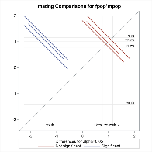
The PLOTS= DIFFPLOT option in the first LSMEANS statement requests a comparison plot that displays the result of all pairwise comparisons (Output 45.2.10). The SLICEDIFF =(mpop fpop) option requests differences of simple effects.
The comparison plot in Output 45.2.10 is also known as a mean-mean scatter plot (Hsu 1996). Each solid line in the plot corresponds to one of the possible  unique pairwise comparisons. The line is centered at the intersection of two least squares means, and the length of the line
segments corresponds to the width of a 95% confidence interval for the difference between the two least squares means. The
length of the segment is adjusted for the rotation. If a line segment crosses the dashed 45-degree line, the comparison between
the two factor levels is not significant; otherwise, it is significant. The horizontal and vertical axes of the plot are drawn
in least squares means units, and the grid lines are placed at the values of the least squares means.
unique pairwise comparisons. The line is centered at the intersection of two least squares means, and the length of the line
segments corresponds to the width of a 95% confidence interval for the difference between the two least squares means. The
length of the segment is adjusted for the rotation. If a line segment crosses the dashed 45-degree line, the comparison between
the two factor levels is not significant; otherwise, it is significant. The horizontal and vertical axes of the plot are drawn
in least squares means units, and the grid lines are placed at the values of the least squares means.
The six pairs of least squares means comparisons separate into two sets of three pairs. Comparisons in the first set are significant; comparisons in the second set are not significant. For the significant set, the female partner in one of the pairs is a whiteside salamander. For the nonsignificant comparisons, the male partner in one of the pairs is a whiteside salamander.
Output 45.2.10: LS-Means Diffogram
The "Simple Effect Comparisons" tables show the results of the SLICEDIFF= option in the second LSMEANS statement (Output 45.2.11).
Output 45.2.11: Simple Effect Comparisons
The first table of simple effect comparisons holds fixed the level of the mpop factor and compares the levels of the fpop factor. Because there is only one possible comparison for each male population, there are two entries in the table. The first
entry compares the logits of mating probabilities when the male partner is a rough butt, and the second entry applies when
the male partner is from the whiteside population. The second table of simple effects comparisons applies the same logic,
but holds fixed the level of the female partner in the pair. Note that these four comparisons are a subset of all six possible
comparisons, eliminating those where both factors are varied at the same time. The simple effect comparisons show that there
is no difference in mating probabilities if the male partner is a whiteside salamander, or if the female partner is a rough
butt. Rough butt females also appear to mate indiscriminately.